Figures & data
Figure 1. Geometry of the inverse problem under investigation.
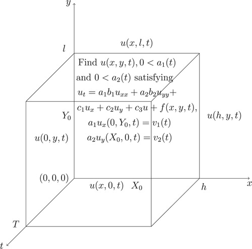
Figure 2. The exact (Equation29(29)
(29) ) and numerical solutions for (a)
and (b)
, with
and with various numbers of time steps
, for direct problem.
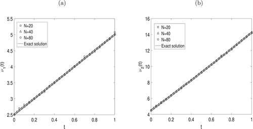
Table 1. The rmse values ((Equation32 (32) (32) ) and (Equation33(33) (33) )) for and , with and with various , for direct problem.
Figure 3. The objective function (Equation19(19)
(19) ), as a function of the number of iterations, for Example 1 with
noise.
![Figure 3. The objective function (Equation19(19) F(a1,a2)=∑n=1N[a1nux(0,Y0,tn)−ν1(tn)]2+∑n=1N[a2nuy(X0,0,tn)−ν2(tn)]2,(19) ), as a function of the number of iterations, for Example 1 with p∈{0,1%,3%,5%} noise.](/cms/asset/5cae5cf9-a60f-4f18-9376-4cb3dac8c288/gipe_a_1814282_f0003_ob.jpg)
Figure 4. The exact (Equation31(31)
(31) ) and numerical solutions for: (a)
and (b)
, for Example 1 with
noise.
![Figure 4. The exact (Equation31(31) a1(t)=1+t,a2(t)=1+2t,t∈[0,1].(31) ) and numerical solutions for: (a) a1(t) and (b) a2(t), for Example 1 with p∈{0,1%,3%,5%} noise.](/cms/asset/1a9f41ab-7600-4c44-aa74-6ec3a73fb435/gipe_a_1814282_f0004_ob.jpg)
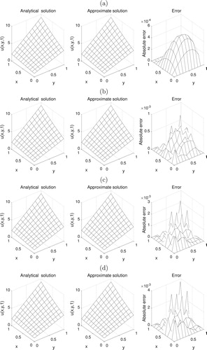
Figure 5. The analytical (Equation30(30)
(30) ) and approximate solutions for the temperature
, for Example 1 with (a) no noise, (b)
noise, (c)
noise, and (d)
noise. The absolute error between them is also included.
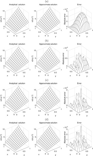
Table 2. The number of iterations, the values of the objective function (19) at final iteration, the rmse values ((26) and (27)) and the computational time, for , for Examples 1 and 2.
Figure 6. The objective function (Equation19(19)
(19) ), as a function of the number of iterations, for Example 2 with
noise.
![Figure 6. The objective function (Equation19(19) F(a1,a2)=∑n=1N[a1nux(0,Y0,tn)−ν1(tn)]2+∑n=1N[a2nuy(X0,0,tn)−ν2(tn)]2,(19) ), as a function of the number of iterations, for Example 2 with p∈{0,1%,3%,5%} noise.](/cms/asset/296b85d8-7779-4fb7-a6b4-ae25021b8f0b/gipe_a_1814282_f0006_ob.jpg)
Figure 7. The exact (Equation35(35)
(35) ) and numerical solutions for: (a)
and (b)
, for Example 2 with
noise.
![Figure 7. The exact (Equation35(35) a1(t)=1+cos2(2πt),a2(t)=1+cos2(3πt),t∈[0,1].(35) ) and numerical solutions for: (a) a1(t) and (b) a2(t), for Example 2 with p∈{0,1%,3%,5%} noise.](/cms/asset/f4330a8a-b678-4ab1-ba68-688209b4eb16/gipe_a_1814282_f0007_ob.jpg)
Figure 8. The analytical (Equation30(30)
(30) ) and approximate solutions for the temperature
, for Example 2 with (a) no noise, (b)
noise, (c)
noise, and (d)
noise. The absolute error between them is also included.