A homogenization function technique to solve the 3D inverse Cauchy problem of elliptic type equations in a closed walled shell

Figures & data

Figure 1. A schematic plot of 3D inverse Cauchy problem in a closed walled shell.

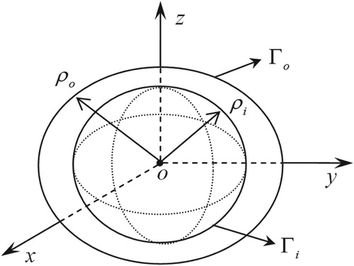
Figure 2. For Example 5.1, comparing (a) numerically recovered and (b) exact boundary data on inner surface.

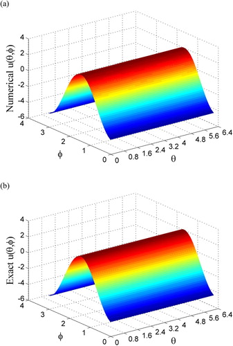
Figure 3. For Example 5.2, comparing (a) numerically recovered and (b) exact boundary data on an inner sphere.

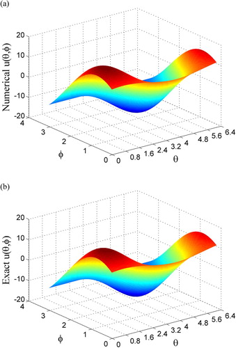
Table 1. For Example 5.2, comparing the maximum error (ME), $e(u)$, the CPU time and the number of steps (No. Steps) for different levels of noise.

Noise	$1\mathrm{\%}$	$5\mathrm{\%}$	$10\mathrm{\%}$	$15\mathrm{\%}$	$20\mathrm{\%}$
ME	0.374	0.379	0.386	0.393	0.399
$e(u)$	$4.970\times {10}^{-4}$	$4.975\times {10}^{-4}$	$4.981\times {10}^{-4}$	$4.989\times {10}^{-4}$	$4.998\times {10}^{-4}$
CPU time	5.85	5.79	5.65	5.65	5.60
No. Steps	51	56	60	63	64

Table 2. For Example 5.2, comparing the ME and CPU time by using the BEM and the present method with various noise levels.

BEM [35]
Noise level	$1\mathrm{\%}$	$3\mathrm{\%}$	$5\mathrm{\%}$
ME	$3.28\times {10}^{-1}$	$5.36\times {10}^{-1}$	$5.15\times {10}^{-1}$
CPU time	112.23	112.11	112.57
Present method
ME	$3.74\times {10}^{-1}$	$3.77\times {10}^{-1}$	$3.79\times {10}^{-1}$
CPU time	5.85	5.41	5.79

Figure 4. For Example 5.3, (a) comparing numerically recovered and exact boundary data on a curve, (b) showing error, and (c) showing error on inner surface.

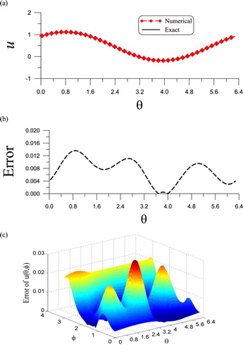
Table 3. For Example 5.3, comparing the maximum error (ME), $e(u)$, the CPU time and the number of steps (No. Steps) for different levels of noise.

Noise	$1\mathrm{\%}$	$5\mathrm{\%}$	$10\mathrm{\%}$	$15\mathrm{\%}$	$20\mathrm{\%}$
ME	$3.079\times {10}^{-2}$	$2.987\times {10}^{-2}$	$3.964\times {10}^{-2}$	$2.944\times {10}^{-2}$	$2.926\times {10}^{-2}$
$e(u)$	$4.091\times {10}^{-4}$	$4.026\times {10}^{-4}$	$4.916\times {10}^{-4}$	$3.913\times {10}^{-4}$	$3.878\times {10}^{-4}$
CPU time	1.15	1.17	1.15	1.15	1.15
No. Steps	19	19	19	19	19

Figure 5. For Example 5.4, (a) comparing numerically recovered and exact boundary data on a curve, (b) showing error, and (c) showing error on inner surface.

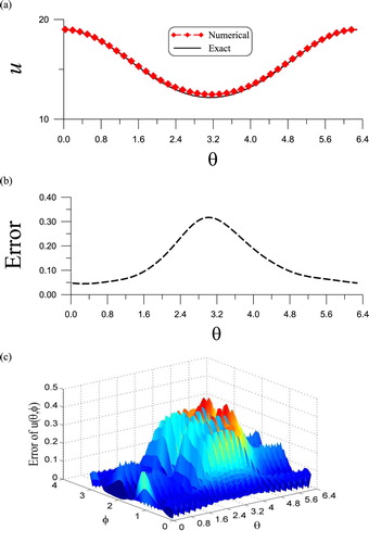
Table 4. For Example 5.4, comparing the maximum error (ME), $e(u)$, and the number of steps (No. Steps) for different values of $R_0$.

$R_0$	$s_{ijk}=1$	10	1	0.1	0.01	0.001
ME	1.228	0.808	0.808	0.808	0.808	0.796
$e(u)$	$1.270\times {10}^{-4}$	$9.007\times {10}^{-5}$	$9.007\times {10}^{-5}$	$9.007\times {10}^{-5}$	$9.007\times {10}^{-5}$	$8.897\times {10}^{-5}$
No. Steps	over 5000	538	485	436	409	327

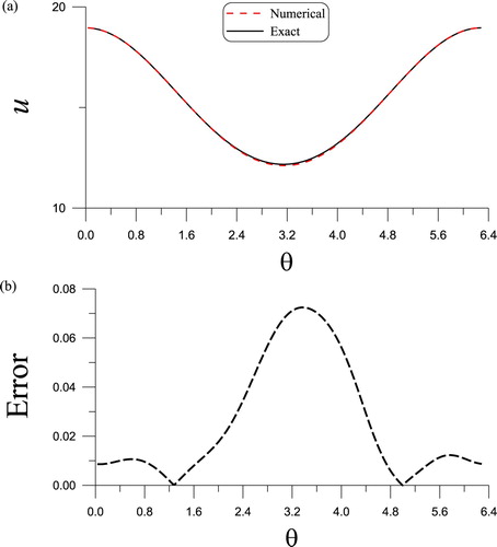
Figure 6. For Example 5.5, (a) comparing numerically recovered and exact boundary data on a curve, and (b) showing error.

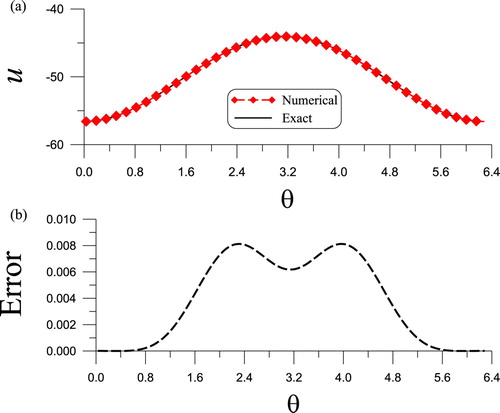
Figure 7. For Example 5.5, comparing (a) numerically recovered and (b) exact boundary data on inner surface.

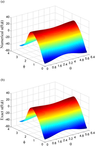
Table 5. For Example 5.5, comparing the maximum error (ME), $e(u)$, the CPU time and the number of steps (No. Steps) for different levels of noise.

Noise	$1\mathrm{\%}$	$5\mathrm{\%}$	$10\mathrm{\%}$	$15\mathrm{\%}$	$20\mathrm{\%}$
ME	$2.648\times {10}^{-2}$	$2.968\times {10}^{-2}$	$3.310\times {10}^{-2}$	$3.666\times {10}^{-2}$	$3.738\times {10}^{-2}$
$e(u)$	$1.046\times {10}^{-5}$	$1.099\times {10}^{-5}$	$1.169\times {10}^{-5}$	$1.272\times {10}^{-5}$	$1.371\times {10}^{-5}$
CPU time	25.56	25.67	25.58	25.50	25.34
No. Steps	317	317	319	319	311

Figure 8. For Example 5.6, (a) convergence rate, (b) comparing numerically recovered and exact boundary data on a curve, and (c) showing error.

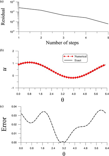
Figure 9. For Example 5.7, (a) comparing numerically recovered and exact boundary data on a curve, and (b) showing error.

Table 6. For Example 5.7, comparing the maximum error (ME), $e(u)$, and the number of steps (No. Steps) for different values of $R_0$.

$R_0$	10	1	0.1	0.01	0.001	0.0001
ME	0.248	0.248	0.248	0.249	0.243	0.276
$e(u)$	$2.662\times {10}^{-5}$	$2.662\times {10}^{-5}$	$2.662\times {10}^{-5}$	$2.658\times {10}^{-5}$	$2.627\times {10}^{-5}$	$2.687\times {10}^{-5}$
No. Steps	1111	1048	1002	879	666	458

Wang F, Chen W, Qu W, et al. A BEM formulation in conjunction with parametric equation approach for three-dimensional Cauchy problems of steady heat conduction. Eng Anal Bound Elem. 2016;63:1–14. doi: 10.1016/j.enganabound.2015.10.007

 Google Scholar