Figures & data
Figure 1. Geometry of Compton scattering: the incident photon energy yields a part of its energy to an electron and is scattered with an angle ω.
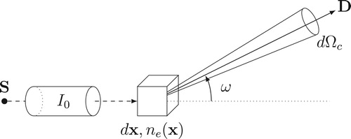
Figure 2. Working principle of systems on 3D CSI.
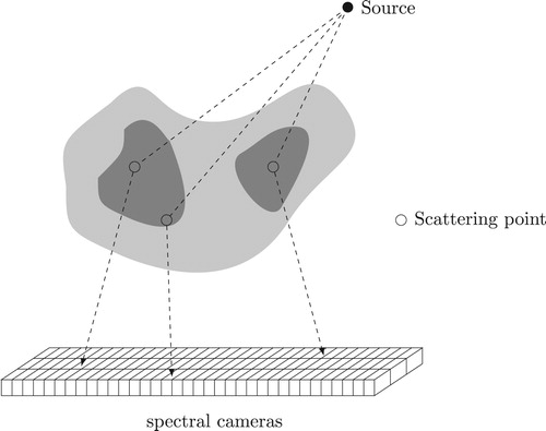
Figure 3. A complete spindle torus (left), its inside part often called lemon (middle) and its outside part often called apple (right) for a given scattering angle . The lemon (middle) represents the torus
whereas the apple (right) represents the torus
.
![Figure 3. A complete spindle torus (left), its inside part often called lemon (middle) and its outside part often called apple (right) for a given scattering angle ω∈[0,π/2]. The lemon (middle) represents the torus T(θ,Eω), whereas the apple (right) represents the torus T(θ,Eπ−ω).](/cms/asset/0cbc0088-95d2-4b4d-b994-5030c82ba999/gipe_a_1815723_f0003_ob.jpg)
Figure 4. A geometric representation of the parametrization of the torus.
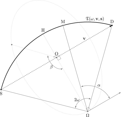
Figure 5. Two configurations for CSI modalities. (a) CSI; (b) CSI
.
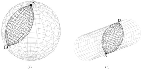
Figure 6. for
.
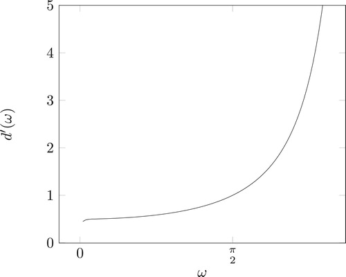
Figure 7. Industrial toy object. First row: central slices of . Second row: central slices of the prior attenuation map used to initialize the projection matrix in cm
.
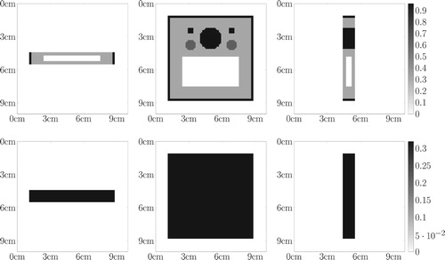
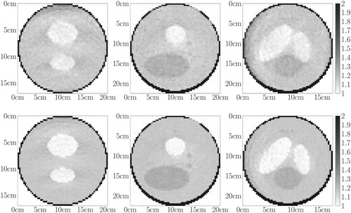
Figure 8. Medical toy object. First row: central slices of . Second row: central slices of the exact attenuation map in cm
. Third row: central slices of the prior attenuation map in cm
used to initialize the projection matrix.
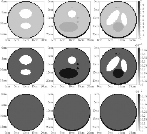
Figure 9. 3D CSI Data – First row depicts the data for the board phantom: (first column) 3D visualization via parallel slices, (columns 2,3,4) corresponding parallel slices. Second row depicts the data for the Shepp–Logan phantom: (first column) 3D visualization via parallel slices, (columns 2,3,4) corresponding parallel slices The greyscale (colourbar) indicates the number of detected photons, the more, the darker.
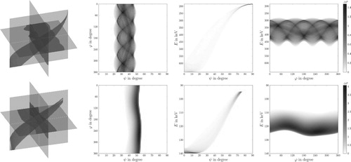
Figure 10. Central slices of the 3D contour reconstruction for the board phantom: first row – with full data, second row – with incomplete data. The intensities are rescaled dividing by .
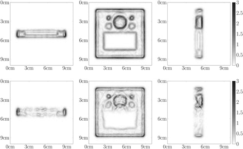
Figure 11. Central slices of the 3D reconstruction for the board phantom: first row – before the TV-denoising step, second row – after the TV-denoising step. The intensities are rescaled dividing by
.
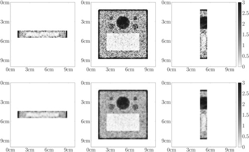
Figure 12. Central slices of the 3D reconstruction for the Shepp–Logan phantom: first row – first iteration of the modified OSEM algorithm after the TV-denoising step, second row – third iteration of the modified OSEM algorithm after the TV-denoising step. The intensities are rescaled dividing by
.
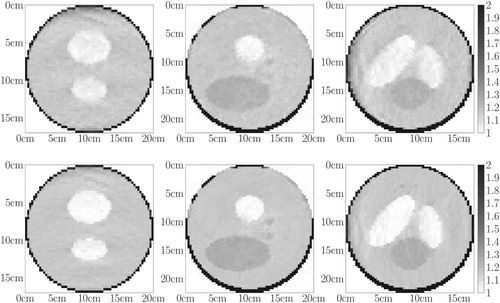
Figure 13. 3D CSI Data – First row depicts the data for the board phantom: (first column) 3D visualization via parallel slices, (columns 2,3,4) corresponding parallel slices. Second row depicts the data for the Shepp–Logan phantom: (first column) 3D visualization via parallel slices, (columns 2,3,4) corresponding parallel slices The greyscale (colourbar) indicates the number of detected photons, the more, the darker.
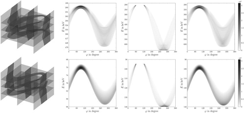
Figure 14. Central slices of the 3D reconstruction for the board phantom: first row – first iteration of the modified OSEM algorithm before the TV-denoising step, second row – fifth iteration of the modified OSEM algorithm before the TV-denoising step, third row – fifth iteration of the modified OSEM algorithm after the TV-denoising step. The intensities are rescaled dividing by
.
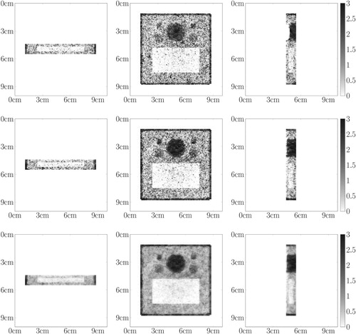
Figure 15. Central slices of the 3D reconstruction for the Shepp–Logan phantom: first row – first iteration of the modified OSEM algorithm after the TV-denoising step, second row – third iteration of the modified OSEM algorithm after the TV-denoising step. The intensities are rescaled dividing by
.