Time-dependent lowest term estimation in a 2D bioheat transfer problem with nonlocal and convective boundary conditions

Figures & data

Figure 1. Domain for perfusion estimation.

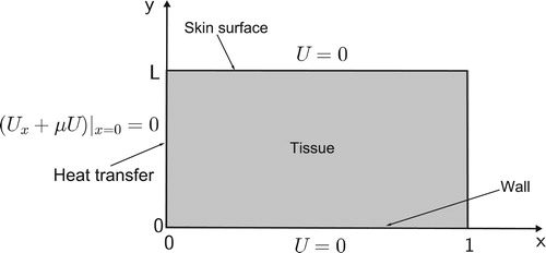
Figure 2. Exact solution and numerical solution of model (1(1) $U_t=U_{xx}+U_{yy}-p\left(t\right)U(x,y,t)+f(x,y,t),(x,y,t)\in ]0,1[\times ]0,L[\times ]0,\mathcal{T}],$(1) )and corresponding error.

Figure 3. Left: Energy values and their Chebyshev-Clenshaw–Curtis based approximations. Right: Pointwise error.

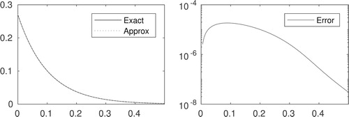
Figure 4. Comparison of quadrature rules efficiency. The error for Clenshaw–Curtis and Gaussian quadrature rules are labelled by Error CC and Error Gauss, respectively.

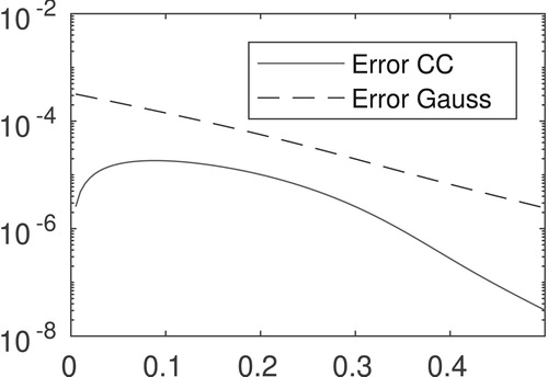
Figure 5. Left: Exact and noisy data for numerical inversion. Noisy data in this illustration corresponds to noise level $1\mathrm{\%}$. Right: Exact coefficient $p\left(t\right)$ and recovered ones.

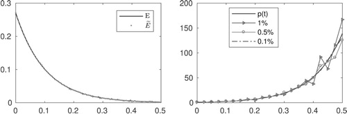
Table 1. Relative error in reconstructing $p\left(t\right)$.

NL	1%	0.5%	0.01%
RE	0.2535	0.1318	0.0344

Figure 6. Exact and recovered temperatures and corresponding pointwise error.

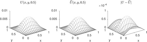
Figure 7. Left: Exact and noisy data for numerical inversion. Noisy data in this illustration corresponds to noise level $1\mathrm{\%}$. Right: Exact coefficient $p\left(t\right)$ and recovered ones.

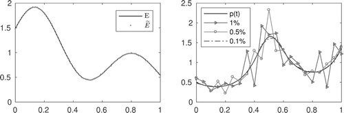
Table 2. Relative error in reconstructing $p\left(t\right)$.

NL	1%	0.5%	0.01%
RE	0.3130	0.041	0.0364

Figure 8. Exact and recovered temperatures and corresponding pointwise error.

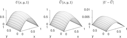
Figure 9. Exact and perturbed initial temperatures and exact and perturbed perfusion coefficient.

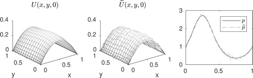
Figure 10. Initial condition, predicted temperature at t = 0.5 and calculated energy.

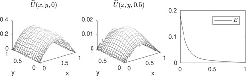
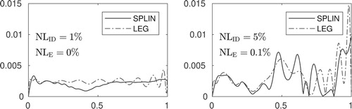
Figure 11. Exact coefficient $p\left(t\right)$ and recovered ones.

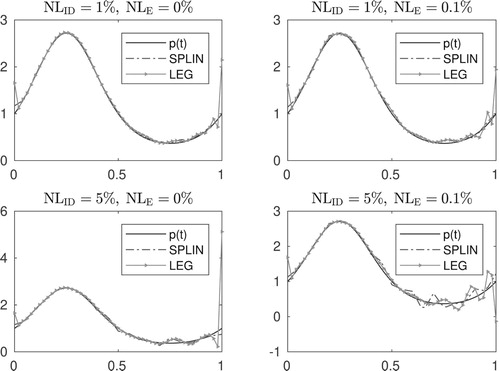
Table 3. Relative error in estimated coefficients.

Case	(S,S)	(S,L)	(L,S)	(L,L)
SPLIN	0.019971	0.025204	0.048042	0.063594
LEG	0.067864	0.067181	0.217524	0.124550

Figure 12. Relative errors in predicted temperatures with recovered coefficient as input data.