Nonlocal viscoelastic Euler-Bernoulli beam model: a Bayesian approach for parameter estimation using the delayed rejection adaptive metropolis algorithm

Figures & data

Table 1. Basic mechanical and geometrical properties of the SWCNT.

Property	Symbol	Value
Length (nm)	l	10
Mid-surface diameter (nm)	d	1
Effective wall thickness (nm)	h	0.342
Mass density (kg/m${}^3$)	ρ	2240
Viscous damping coefficient (Ns/m)	C	0
Static modulus (TPa)	$E_{\mathrm{\infty }}$	1

Table 2. First three undamped natural frequencies of the local model ($e_{0}a=0$ and $\mathrm{\Delta }=0$).

Mode	${\omega }_r^{\prime }$ (GHz)
1	124.01
2	496.06
3	1116.16

Table 3. Nonlocal and viscoelastic parameters adopted for the parametric analysis of the undamped natural frequencies and damping ratios.

Property	Symbol	Value
Nonlocal parameter (nm)	$e_{0}a$	$\in [0;2]$
Relaxation modulus	Δ	0.5
Inverse of relaxation time (rad/s)	Ω	$\in [0.01;100]\times {10}^{12}$

Figure 1. Nonlocal and viscoelastic effects on the first normalized undamped natural frequency ${\omega }_1/{\omega }_1^{\prime }$ (a) and damping ratio ${\zeta }_1$ (b).

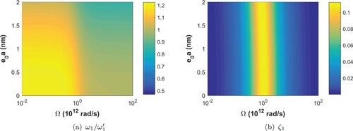
Figure 2. Nonlocal and viscoelastic effects on the second normalized undamped natural frequency ${\omega }_2/{\omega }_2^{\prime }$ (a) and damping ratio ${\zeta }_2$ (b).

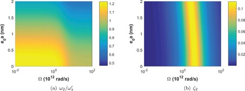
Figure 3. Nonlocal and viscoelastic effects on the third normalized undamped natural frequency ${\omega }_3/{\omega }_3^{\prime }$ (a) and damping ratio ${\zeta }_3$ (b).

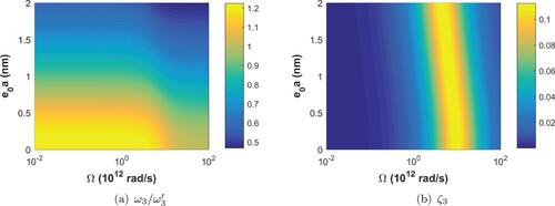
Table 4. Viscoelastic and nonlocal parameters adopted in the inverse problems of Cases 1 and 2.

Property	Symbol	Value
Nonlocal parameter (nm)	$e_{0}a$	1.5
Relaxation resistance	Δ	0.5
Inverse of relaxation time (rad/s)	Ω	$0.4\times {10}^{12}$

Table 5. Reference values for the undamped natural frequencies and damping ratios for Cases 1 and 2.

Mode	${\omega }_r$ (GHz)	${\zeta }_r$
1	134.25	0.072
2	441.12	0.024
3	788.86	0.013

Note: These modal parameters were computed considering the properties shown in Tables 1 and 4.

Table 6. Cases 1 and 2 addressed in the inverse problem of parameter estimation.

		Diameter nominal	Unknown parameter
Case		value $d_0$ (nm)	vector ($\mathit{\theta }$)
	A	1.00
1	B	0.97	$[e_{0}a,\mathrm{\Delta },\mathrm{\Omega }{]}^T$
	C	1.03
	A	1.00
2	B	0.97	$[e_{0}a,\mathrm{\Delta },\mathrm{\Omega },d{]}^T$
	C	1.03

Figure 4. (a) Markov Chains and (b) Marginal PDFs for $e_{0}a$ – Cases 1A, 1B and 1C. Note: dashed lines indicate the reference value.

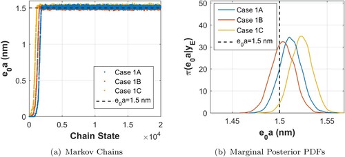
Figure 6. (a) Markov Chains and (b) Marginal PDFs for Ω – Cases 1A, 1B and 1C. Note: dashed lines indicate the reference value.

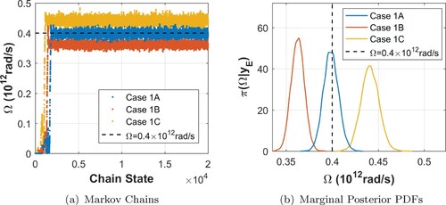
Figure 5. (a) Markov Chains and (b) Marginal PDFs for Δ – Cases 1A, 1B and 1C. Note: dashed lines indicate the reference value.

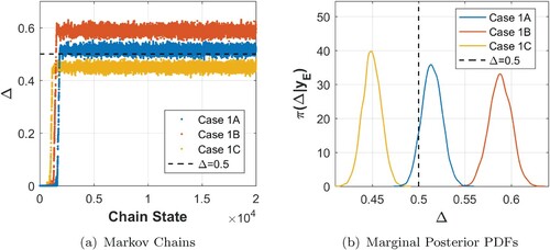
Table 7. Parameter estimation results: Cases 1A, 1B and 1C.

Case	Parameter	Exact value	μ	σ	$\sigma /\mu$ $\mathrm{\%}$	CI 95$\mathrm{\%}$	MAP
	$e_{0}a$ (nm)	1.5	1.512	0.012	0.77	[1.489, 1.535]	1.512
1A	Δ	0.5	0.515	0.011	2.09	[0.494, 0.536]	0.515
	Ω (${10}^{12}$ rad/s)	0.4	0.399	0.008	2.03	[0.383, 0.415]	0.398
	$e_{0}a$ (nm)	1.5	1.504	0.012	0.80	[1.480, 1.527]	1.503
1B	Δ	0.5	0.588	0.012	2.02	[0.565, 0.611]	0.588
	Ω (${10}^{12}$ rad/s)	0.4	0.363	0.007	1.96	[0.349, 0.377]	0.363
	$e_{0}a$ (nm)	1.5	1.523	0.011	0.74	[1.501, 1.545]	1.523
1C	Δ	0.5	0.450	0.010	2.22	[0.430, 0.469]	0.449
	Ω (${10}^{12}$ rad/s)	0.4	0.441	0.010	2.17	[0.423, 0.460]	0.441

Figure 7. Marginal posterior distributions (diagonal plots) and scatter plots of model parameters - Cases 1A, 1B and 1C.

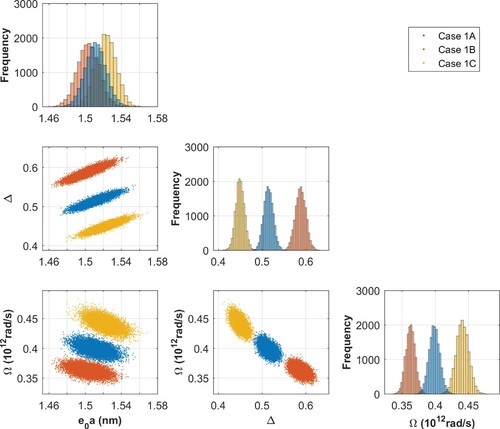
Figure 8. (a) Markov Chains and (b) Marginal PDFs for $e_{0}a$ – Cases 2A, 2B and 2C. Note: dashed lines indicate the reference value.

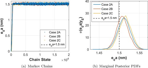
Figure 9. (a) Markov Chains and (b) Marginal PDFs for Δ – Cases 2A, 2B and 2C. Note: dashed lines indicate the reference value.

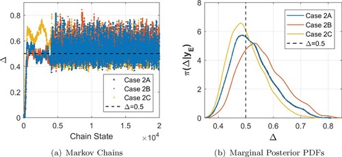
Figure 10. (a) Markov Chains and (b) Marginal PDFs for Ω – Cases 2A, 2B and 2C. Note: dashed lines indicate the reference value.

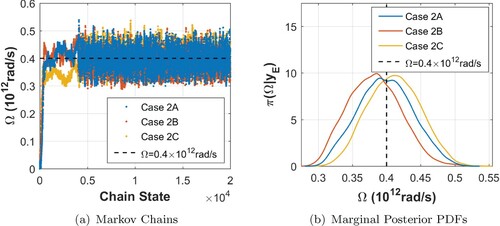
Figure 11. (a) Markov Chains and (b) Marginal PDFs for d – Cases 2A, 2B and 2C. Note: dashed lines indicate the reference value.

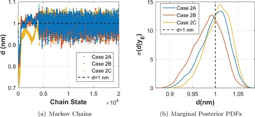
Figure 12. Marginal posterior distributions (diagonal plots) and scatter plots of model parameters – Cases 2A, 2B and 2C.

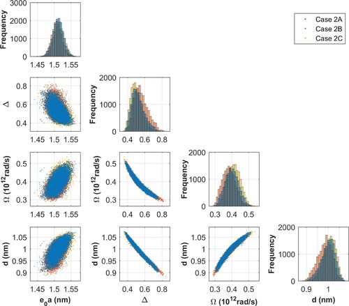
Table 8. Parameter estimation results: Cases 2A, 2B and 2C.

Case	Parameter	Exact value	μ	σ	$\sigma /\mu$ $\mathrm{\%}$	CI 95$\mathrm{\%}$	MAP
	$e_{0}a$ (nm)	1.5	1.512	0.016	1.02	[1.481, 1.542]	1.513
2A	Δ	0.5	0.524	0.073	13.91	[0.409, 0.695]	0.508
	Ω (${10}^{12}$ rad/s)	0.4	0.399	0.039	9.84	[0.325, 0.476]	0.403
	d (nm)	1.0	0.998	0.030	3.04	[0.931, 1.049]	1.003
	$e_{0}a$ (nm)	1.5	1.508	0.015	0.98	[1.480, 1.537]	1.509
2B	Δ	0.5	0.558	0.079	14.22	[0.429, 0.732]	0.537
	Ω (${10}^{12}$ rad/s)	0.4	0.382	0.038	9.95	[0.314, 0.459]	0.387
	d (nm)	1.0	0.984	0.036	3.20	[0.919, 1.038]	0.991
	$e_{0}a$ (nm)	1.5	1.515	0.015	0.98	[1.486, 1.544]	1.517
2C	Δ	0.5	0.503	0.064	12.74	[0.401, 0.647]	0.485
	Ω (${10}^{12}$ rad/s)	0.4	0.411	0.038	9.17	[0.340, 0.485]	0.417
	d (nm)	1.0	1.006	0.027	2.73	[0.947, 1.053]	1.013

Table 9. Viscoelastic and nonlocal parameters adopted to generate the synthetic data in Case 3.

Property	Symbol	Value
Nonlocal parameter (nm)	$e_{0}a$	1.5
Relaxation resistance 1	${\mathrm{\Delta }}_1$	0.5
Inverse of relaxation time 1 (rad/s)	${\mathrm{\Omega }}_1$	$0.4\times {10}^{12}$
Relaxation resistance 2	${\mathrm{\Delta }}_2$	0.5
Inverse of relaxation time 2 (rad/s)	${\mathrm{\Omega }}_2$	$6.3\times {10}^{12}$

Table 10. Reference values for the undamped natural frequencies and damping ratios for Case 3.

Mode	${\omega }_r$ (GHz)	${\zeta }_r$
1	135.11	0.095
2	455.56	0.085
3	847.97	0.089

Note: These modal parameters were computed considering the properties shown in Tables 1 and 9.

Table 11. Case 3 addressed in the inverse problem of parameter estimation.

	Diameter nominal	Unknown parameter
Case	value $d_0$ (nm)	vector ($\mathit{\theta }$)
3	1.00	$[e_{0}a,\mathrm{\Delta },\mathrm{\Omega },d,\beta {]}^T$

Figure 13. Marginal posterior distributions (diagonal plots) and scatter plots of model parameters – Case 3.

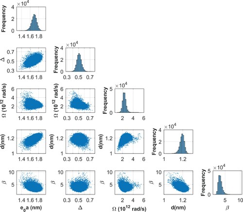
Table 12. Parameter estimation results: Case 3.

Parameter	Exact value	μ	σ	$\sigma /\mu$ $\mathrm{\%}$	CI 95$\mathrm{\%}$	MAP
$e_{0}a$ (nm)	1.5	1.694	0.059	3.50	[1.568, 1.804]	1.713
Δ	–	0.511	0.040	7.75	[0.436, 0.592]	0.512
Ω (${10}^{12}$ rad/s)	–	2.335	0.312	13.34	[1.788, 3.011]	2.322
d (nm)	1	1.193	0.023	1.93	[1.143, 1.234]	1.201
β	–	3.398	0.630	18.53	[2.456, 4.864]	2.871

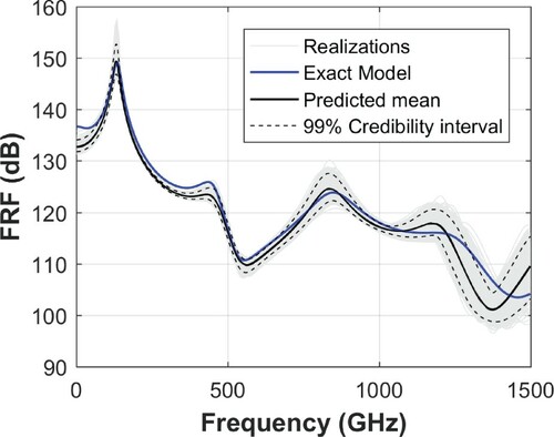
Figure 14. Frequency Response Function of the reference model along with the mean and 99% credibility interval predicted by the model used in the inversion.