A high order PDE-constrained optimization for the image denoising problem

Figures & data

Figure 1. Plot of the PSNR values of the restored image using the TGV and TV+TV${}^2$ approach with respect to the parameters ${\alpha }_0$ and ${\alpha }_1$. We can see that the highest achieved PSNR for the TGV${}^2$ approach is related to the values ${\alpha }_0=0.06$ and ${\alpha }_0=0.04$. For the TV+TV${}^2$ model, the best PSNR corresponds to the values ${\alpha }_0=0.011$ and ${\alpha }_0=0.05$. Note that the original image is the Pirate one corrupted by Gaussian noise of variance 0.3.

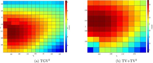
Figure 2. The obtained denoised image compared to other classical approaches for the (Pirate image), where the noise is considered to be Gaussian of $\sigma =0.3$: (a) Noisy image, (b) ROF model [3], (c) NLM model [51], (d) TV+TV${}^2$ [19] (e) TGV model [36] and (f) Our model.

Figure 3. The obtained denoised image compared to other classical approaches for the (Cameraman image), where the noise is considered to be Gaussian of $\sigma =0.5$: (a) Noisy image, (b) ROF model [3], (c) NLM model [51], (d) TV+TV${}^2$ [19], (e) TGV model [36] and (f) our model.

Figure 4. The computation of the parameter λ with respect to the iteration for the two images Pirate and Cameraman: (a) The Pirate image and (b) The Cameraman image.

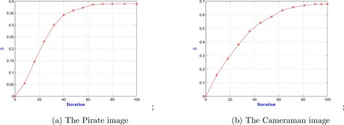
Figure 5. The obtained denoised image compared to other classical approaches for the Cameraman image, where the noise is considered to be impulse one of parameter 0.3: (a) Noisy image, (b) ROF [3], (c) NLM [51], (d) L${}^1$-TV+TV${}^2$ [19], (e) L${}^1$-TGV [36] and (f) Our model.

Figure 6. The obtained denoised image compared to other classical approaches for the (Penguin image), where the noise is considered to be impulse one of parameter 0.5: (a) Noisy image, (b) ROF model [3], (c) NLM model [51], (d) L${}^1$-TV+TV${}^2$ [19], (e) L${}^1$-TGV model [36] and (f) Our model.

Figure 7. The computation of the parameter λ with respect to the iteration for the two images Camerman and Penquin: (a) The Pirate image and (b) The Penguin image.

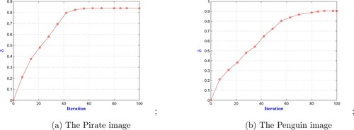
Table 1. The PSNR table.

Image	PSNR
	ROF model [3]	NLM model [51]	TV+TV${}^2$ [19]	TGV model [36]	Our Method
Pirate (Gaussian noise with $\sigma =0.3$)	27.40	28.02	28.88	29.50	$\mathbf{\text{29.88}}$
Cameraman (Gaussian noise with $\sigma =0.5$)	26.90	27.25	28.02	28.28	$\mathbf{\text{29.01}}$
Penguin (impulse noise with parameter 0.3)	23.07	23.80	24.65	$\mathbf{\text{25.11}}$	24.82
Cameraman (impulse noise with parameter 0.5)	26.55	27.03	27.81	28.30	$\mathbf{\text{29.05}}$

Table 2. The SSIM table.

Image	SSIM
	ROF model [3]	NLM model [51]	TV+TV${}^2$ [19]	TGV model [36]	Our Method
Pirate (Gaussian noise with $\sigma =0.3$)	0.886	0.883	0.896	0.902	$\mathbf{\text{0.922}}$
Cameraman (Gaussian noise with $\sigma =0.5$)	0.701	0.707	0.737	0.745	$\mathbf{\text{0.784}}$
Penguin (impulse noise with parameter 0.3)	0.662	0.633	0.698	0.730	$\mathbf{\text{0.738}}$
Cameraman (impulse noise with parameter 0.5)	0.683	0.672	0.763	0.809	$\mathbf{\text{0.814}}$

Table 3. The normalized ${\mathit{l}}^{\mathit{2}}$ distance table.

Image	${\mathit{l}}^{\mathit{1}}$ noise level	$l^2$ distance
		ROF model [3]	NLM model [51]	TV+TV${}^2$ [19]	TGV model [36]	Our Method
Pirate (Gaussian noise with $\sigma =0.3$)	872.4442	351.3230	344.8833	350.1111	341.2931	$\mathbf{\text{307.7933}}$
Cameraman (Gaussian noise with $\sigma =0.5$)	982.3456	522.7418	508.3222	501.6144	498.6666	$\mathbf{\text{473.2997}}$
Penguin (impulse noise with parameter 0.3)	813.1955	612.3734	603.7228	600.6999	587.2444	$\mathbf{\text{576.3333}}$
Cameraman (impulse noise with parameter 0.5)	966.9266	674.6688	669.5133	671.6100	659.0233	$\mathbf{\text{612.9887}}$

Table 4. The normalized ${\mathit{l}}^{\mathit{1}}$ distance table.

Image	${\mathit{l}}^{\mathit{1}}$ noise level	${\mathit{l}}^{\mathit{2}}$ distance
		ROF model [3]	NLM model [51]	TV+TV${}^2$ [19]	TGV model [36]	Our Method
Pirate (Gaussian noise with $\sigma =0.3$)	6.6622e+03	3.3381e+03	2.9363e+03	3.1209e+03	2.7111e+03	$\mathbf{\text{2.5552e+03}}$
Cameraman (Gaussian noise with $\sigma =0.5$)	6.8060e+03	3.4831e+03	3.3332e+03	3.0888e+03	2.9166e+03	$\mathbf{\text{2.7733e+03}}$
Penguin (impulse noise with parameter 0.3)	6.7134e+03	3.5266e+03	3.6001e+03	3.1887e+03	3.30933e+03	$\mathbf{\text{2.9283e+03}}$
Cameraman (impulse noise with parameter 0.5)	7.4333e+03	4.2733e+03	4.5002e+03	4.1666e+03	3.9444e+03	$\mathbf{\text{3.7931e+03}}$

Figure 8. The restored image and the parameter λ using the two admissible sets of the Lena image: (a) Noisy, (b) X using ${\mathcal{U}}_{ad}^2$, (c) λ using ${\mathcal{U}}_{ad}^2$, (d) X using ${\mathcal{U}}_{ad}^1$ and (e) λ using ${\mathcal{U}}_{ad}^1$.

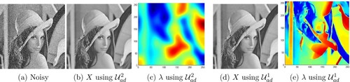
Figure 9. The restored image X and the corresponding weighted parameter λ using the admissible set ${\mathcal{U}}_{ad}^2$. The Baboon image is contaminated by Gaussian noise with $\sigma =0.1$, Penguin image is contaminated by $\sigma =0.3$, Zebra image is contaminated by $\sigma =0.4$, Tiger image is contaminated by $\sigma =0.5$. The used parameters for these tests are: $(k_1,k_2)=(35,89)$, $\sigma =1.3$ and $\rho =2.7$: (a) Noisy, (b) Obtained X, (c) λ and (d) Image of λ.

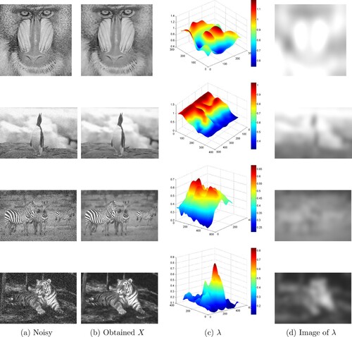
Figure 10. The restored image X and the corresponding weighted parameter λ using the admissible set ${\mathcal{U}}_{ad}^1$. the Baboon image is contaminated by Gaussian noise with $\sigma =0.1$, Penguin image is contaminated by $\sigma =0.3$, Zebra image is contaminated by $\sigma =0.4$, Tiger image is contaminated by $\sigma =0.5$. The used parameters for these tests are: $(k_1,k_2)=(35,80)$, $\sigma =1.7$ and $\rho =2.3$: (a) Noisy, (b) Obtained X, (c) Obtained λ and (d) Image of λ.

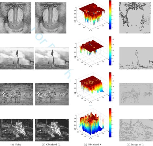
Figure 11. Comparison between the obtained clean image X and the SDRTV method with the respective computation of the spatially dependent parameter λ of the Head image: (a) Original, (b) Noisy, (c) λ initial, (d) SDRTV, (e) Obtained λ, (f) Image of λ, (g) Proposed PDE, (h) Obtained λ and (i) Image of λ.

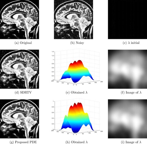
Figure 12. Comparison between the obtained clean image and the SDRTV method and the respective computation of the spatially dependent parameter λ of the Brain image: (a) Original, (b) Noisy, (c) λ initial, (d) SDRTV, (e) Obtained λ, (f) Image of λ, (g) SDRTV, (h) Obtained λ and (i) Image of λ.

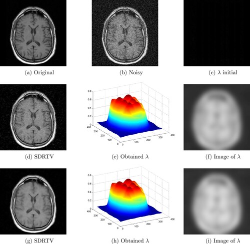
Figure 13. Comparison between the obtained clean image X and the SDRTV method with the respective computation of the spatially dependent parameter λ of the Dolphins image: (a) Original, (b) Noisy, (c) λ initial, (d) SDRTV, (e) Obtained λ, (f) Image of λ, (g) Obtained X, (h) Obtained λ and (i) Image of λ.

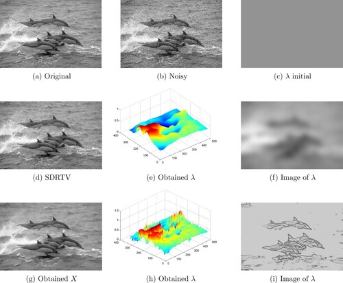
Figure 14. Comparison between the obtained clean image X and the SDRTV method with the respective computation of the spatially-dependent parameter λ of the Plane image: (a) Original, (b) Noisy, (c) λ initial, (d) SDRTV, (e) Obtained λ, (f) Image of λ, (g) Obtained X, (h) Obtained λ and (i) Image of λ.

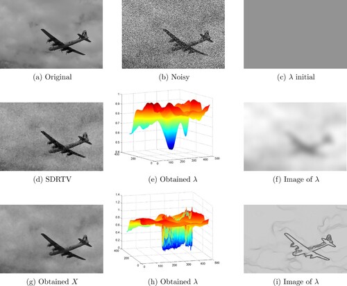
Figure 15. Comparison between the obtained clean image X and the respective computation of the spatially dependent parameter λ for the scalar case and for it two set of admissible values ${\mathcal{U}}_{ad}^1$ and ${\mathcal{U}}_{ad}^2$ for the Fishes image: (a) Original, (b) Noisy, (c) scalar λ, (d) weighted $\lambda \in {\mathcal{U}}_{ad}^2$ and (e) weighted $\lambda \in {\mathcal{U}}_{ad}^1$.

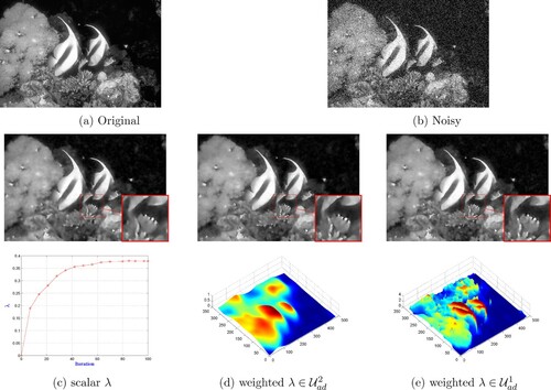
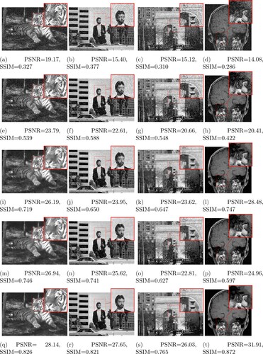
Figure 16. The obtained denoised image compared to other PDE approaches with respect to both quality measures PSNR and SSIM. First row: noisy images. Second row: FOPDE. Third row: AEFD. Fourth row: AFOD. Fifth row: Our approach. (a) PSNR = 19.17, SSIM = 0.327. (b) PSNR = 15.40, SSIM = 0.377. (c) PSNR = 15.12, SSIM = 0.310. (d) PSNR = 14.08, SSIM = 0.286. (e) PSNR = 23.79, SSIM = 0.539. (f) PSNR = 22.61, SSIM = 0.588. (g) PSNR = 20.66, SSIM = 0.548. (h) PSNR = 20.41, SSIM = 0.422, (i) PSNR = 26.19, SSIM = 0.719, (j) PSNR = 23.95, SSIM = 0.650, (k) PSNR = 23.62, SSIM = 0.647. (l) PSNR = 28.48, SSIM = 0.747. (m) PSNR = 26.94, SSIM = 0.746, (n) PSNR = 25.62, SSIM = 0.741, (o) PSNR = 22.81, SSIM = 0.627, (p) PSNR = 24.96, SSIM = 0.597, (q) PSNR = 28.14, SSIM = 0.826, (r) PSNR = 27.65, SSIM = 0.821, (s) PSNR = 26.03, SSIM = 0.765 and (t) PSNR = 31.91, SSIM = 0.872.

Rudin LI, Osher S, Fatemi E. Nonlinear total variation based noise removal algorithms. Phys D Nonlinear Phenom. 1992;60(1-4):259–268.

 Google Scholar

Buades A, Coll B, Morel J-M. Non-local means denoising. Image Process On Line. 2011;1:208–212.

 Google Scholar

Papafitsoros K, Schönlieb C-B. A combined first and second order variational approach for image reconstruction. J Math Imaging Vis. 2014;48(2):308–338.

 Google Scholar

Bredies K, Kunisch K, Pock T. Total generalized variation. SIAM J Imaging Sci. 2010;3(3):492–526.

 Google Scholar