Inverse scattering problem for detecting a defect in a magnetoelastic layer

Figures & data

Table 1. The physical and magnetic properties of used material.

Material	Density (Kg/m${}^3$)	Electrical conductivity (S/m)	Young modulus (N/m2)	Poisson's ratio	Relative permeability (H/m)
Copper	8890	$5.8\times {10}^7$	124 GPa	0.36	0.9999
Copper-Nickel	8500	$2.66\times {10}^6$	120 GPa	0.35	16
Nickel	8300	$1.43\times {10}^7$	190 GPa	0.305	100

Figure 1. The solution of the direct problem for an elliptical defect in three conductive materials, under various strengths of the magnetic field, versus the contour ℓ in degrees.

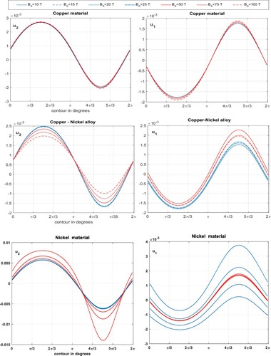
Figure 2. The diffracted surface waves from a defect centred at (1, 1), in three conductive materials, under various strengths of the magnetic field, versus a finite interval on the upper surface.

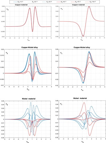
Figure 3. (a) the solution of the direct problem for inclined elliptical defects with three angles $\theta =0,\pi /2,3\pi /4$ in Copper-Nickel material, (b) the solution for smooth rectangular defects with rounded corners in Nickel material, (c) the solution for smooth epicycloidal defects with having different cross-sections.

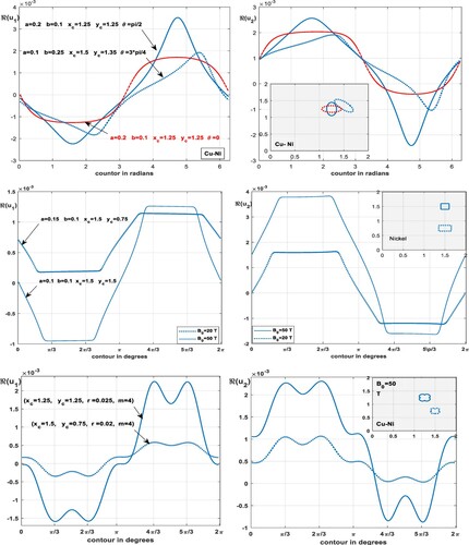
Figure 4. The relative error criterion $|{ϵ}_i|$ of ellipse parameters, in three different materials in the absence of the magnetic field, with the corresponding restored vector x of the parameters.

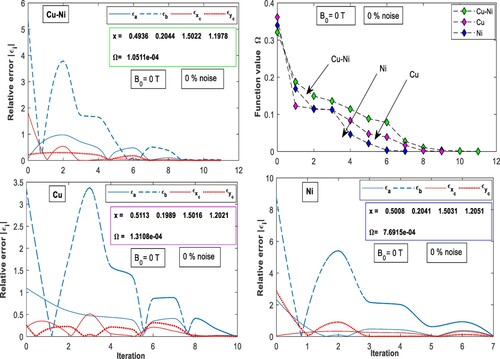
Figure 5. (a) The minimizing path of the discrepancy functional Ω in two noise levels, (b) the relative error criterion $|{ϵ}_i|$ of ellipse parameters in a Copper-Nickel alloy, subjected to a magnetic field of strength 50 Tesla, with the corresponding restored vector x of the parameters.

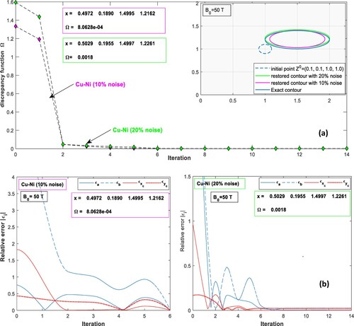
Figure 6. (a) The minimizing path of the discrepancy functional Ω in two noise levels, (b) the relative error criterion $|{ϵ}_i|$ of ellipse parameters in Nickel layer, subjected to a magnetic field of strength 50 Tesla, versus the number of iterations, with the corresponding restored vector x of the parameters.

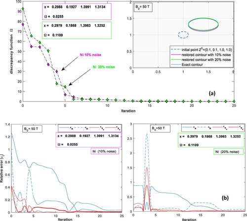
Figure 7. (a) The minimizing path of the discrepancy functional Ω in two noise levels, (b) the relative error criterion $|{ϵ}_i|$ of ellipse parameters, close to bottom of a Copper layer subjected to a magnetic field of strength 100 Tesla, with the corresponding restored vector x of the parameters.

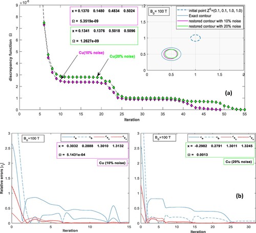
Figure 8. Three noisy levels of minimizing the discrepancy functional Ω, for reconstructing two elliptical defects with inclined angles $\mathrm{\Theta }=\pi /2,3\pi /4$ in a Copper-Nickel layer subjected to an initial magnetic field B${}_0$=50 Tesla, with the corresponding restored vector x of the parameters.

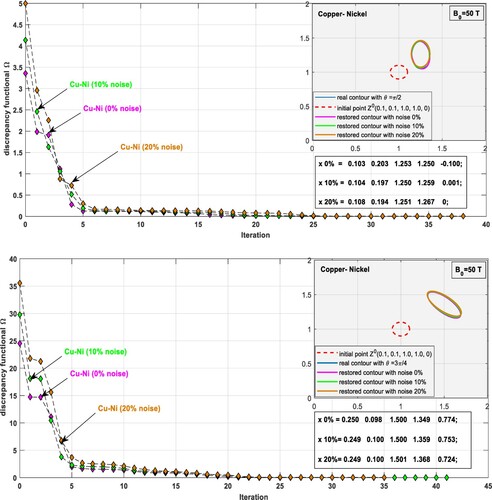
Figure 9. Three noisy levels of the minimizing the discrepancy functional Ω for reconstructing two defects in the shape of a square and rectangle with rounded corners, in a Nickel layer subjected to two different magnetic fields B${}_0$= 20, 50 Tesla, with the corresponding restored vector x of the parameters.

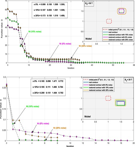
Figure 10. Three noisy levels of minimizing the discrepancy functional Ω for reconstructing two epicycloidal defects, in a Copper-Nickel layer subjected to magnetic field B${}_0$= 50 Tesla, by using rectangular and elliptical shapes, with the corresponding restored vector x of the parameters.

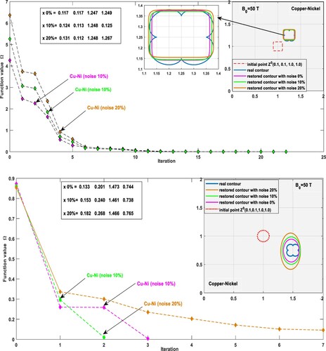
Figure 11. The reconstructing images of an irregular shape with 5 vertices by using elliptical shapes, at different frequencies, in a Copper-Nickel layer subjected to magnetic field B${}_0$= 10 Tesla.

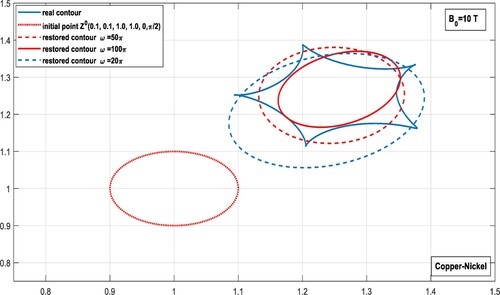
Table 2. Examples of the reconstruction in three different materials, in two noisy cases, under a magnetic field with various strengths versus the relative error criteria.

Material	Noise	B${}_0$	Iteration	${ϵ}_a$%	${ϵ}_b$ %	${ϵ}_{xc}$%	${ϵ}_{yc}$ %	${ϵ}_A$ %
Nickel	5%	20	25	0.20	1.25	0	0.40	1.95
		50	26	0.20	1.90	0.03	0.53	2.10
		100	46	2.4	3. 2	4.5	3.25	4.25
	20%	20	18	0.37	2.50	0.01	1.54	2.88
		50	25	0.70	6.60	0.12	1.94	7.25
		100	81	8.15	10.2	10.31	11.02	18.40
			High relative errors since Ω doesn't converges to zero
Copper Nickel	5%	20	24	0.43	2.25	0.036	0.54	1.73
		50	25	1.50	0.27	0	0.48	1.76
		100	25	6.7	3.60	0	0.62	4.24
	20%	20	23	1.57	8.05	0.14	1.96	6.61
		50	23	0.53	4.85	0.007	1.75	5.36
		100	27	1.97	10.50	0.014	2.13	8.26
Copper	5%	20	24	0.37	2.05	0.05	0.54	1.29
		50	22	0.40	2.10	0.042	0.54	1.31
		100	25	0.50	2.20	0.028	0.54	1.71
	20%	20	25	1.47	7.25	0.18	1.98	4.89
		50	25	1.50	7.35	0.16	1.98	4.96
		100	26	1.77	7.95	0.10	1.98	6.32

Table 3. Examples of prediction of the external magnetic field applied upon a copper layer having different defects.

Material	ℓ (a, b, x${}_c$, y${}_c$)	B${}_0$	Noise	Iteration	Ω value	B*	${ϵ}_B$ %
Copper	(0.2, 0.15, 1.25, 1.20)	125	0%	5	1.9349e-06	122.680	1.71
			10%	10	2.8336e-04	129.7911	3.84
			20%	17	0.00435	133.3201	6.64
	(0.05, 0.05, 1.50, 1.30)	125	0%	8	2.4910e-06	124.866	0.12
			10%	24	1.5336e-04	121. 646	2.72
			20%	17	0.001472	119.3645	4.51
	(0.5, 0.5, 1.0, 1.0)	125	0%	4	1.4628e-06	129.7911	3.84
			10%	9	6.5336e-04	139.105	11.28
			20%	24	0.61252	145	16