
Figures & data
Figure 1. Simulation of a 2D S-shaped duct with balls and spines.
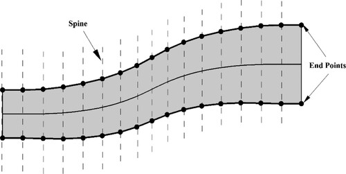
Figure 2. Applying the target and computed pressures on a sample ball.
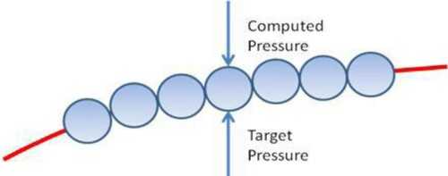
Figure 3. Free-body diagram of a sample ball on the duct wall.
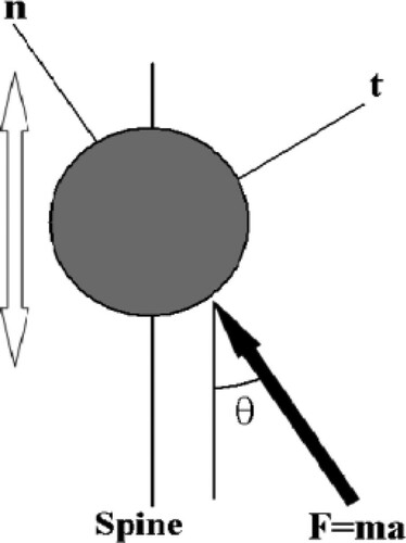
Figure 4. Diagram of ball-spine direction in each cross section.
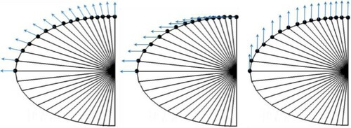
Figure 5. Schematic of force applied to the balls and the different spines for node displacement.
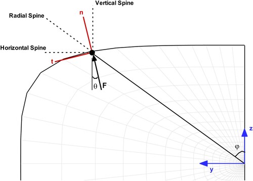
Figure 6. Diagram of geometry with two methods for grid generation.
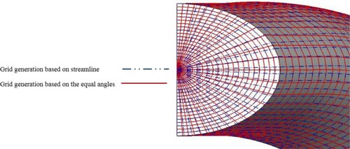
Table 1. Weighting function for SG using second-order polynomial and 5 data points.
Figure 7. Schematic of points used for filtration along the longitudinal and cross-sections.
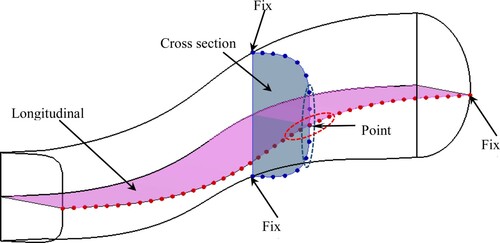
Figure 8. Grid-independency for wall pressure distribution along the upper and lower lines of the symmetric plane.
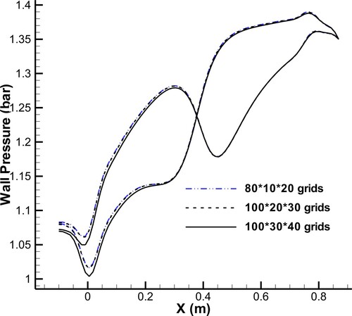
Figure 9. Diagram of cross-sectional design parameters.
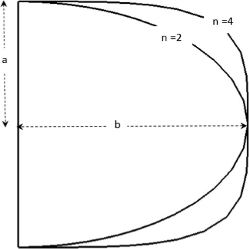
Figure 10. Three geometries with the same centre-line curvature and different cross-sections, and (a) their corresponding pressure distributions along the upper and lower lines of the symmetry plane, and (b) average pressure of cross-section.
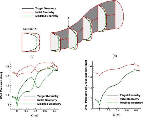
Figure 11. Evolution of geometries and their corresponding pressure distributions from the initial guess to the target geometry.
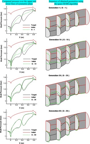
Figure 12. Target geometry and corresponding wall pressure distribution.
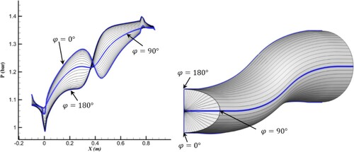
Figure 13. Results of inverse design with similar cross-sectional profiles (n = 2) for the initial and target geometry using an equally angled grid and radial spines after 150 geometry corrections.
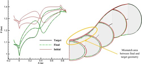
Figure 14. Results of inverse design with similar cross-sectional profiles (n = 4) for the initial and target geometries using an equally angled grid and radial spines after 150 geometry corrections.
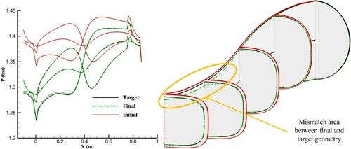
Figure 15. Results of inverse design with different cross-sectional profiles for the initial guess (n = 6) and target geometries (n = 2) using an equally angled grid and radial spines after 150 geometry corrections.
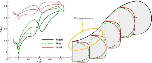
Figure 16. Results of inverse design with different cross-sectional profiles for the initial guess (n = 6) and target geometries (n = 2) using radial spines after 200 geometry corrections.
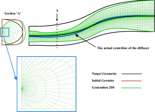
Figure 17. Results of inverse design with similar cross-sectional profiles (n = 2) for the initial and target geometries using an equally angled grid and vertical spines after 200 geometry corrections.
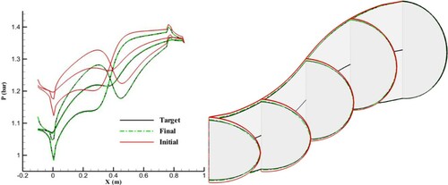
Figure 18. Results of inverse design with similar cross-sectional profiles (n = 4) for the initial and target geometries using an equally angled grid and vertical spines after 200 geometry corrections.
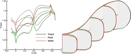
Figure 19. Results of inverse design with different cross-sectional profiles for the initial guess (n = 6) and target geometry (n = 2) using an equally angled grid and vertical spines after 200 geometry corrections.
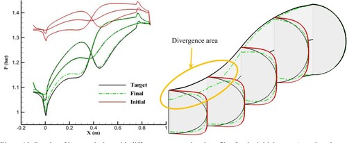
Figure 20. Results of inverse design with similar cross-sectional profiles (n = 2) for the initial and target geometries using an equally angled grid and horizontal spines after 200 geometry corrections.
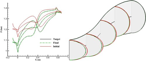
Figure 21. Results of inverse design with similar cross-sectional profiles (n = 4) for the initial and target geometries using an equally angled grid and horizontal spines after 200 geometry corrections.
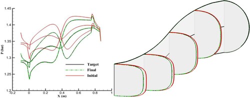
Figure 22. Results of inverse design with different cross-sectional profiles for the initial guess (n = 6) and target geometry (n = 2) using an equally angled grid and horizontal spines.
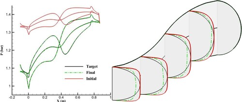
Figure 23. Comparison of wall pressure distributions for the target and final geometry with an equally angled grid along the lateral lines of the wall at various sectors.
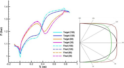
Figure 24. Comparison of streamline-based and equally angled grid generation for the initial guess and target geometry with the same cross-sectional profile.
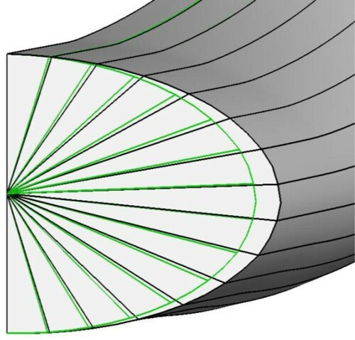
Figure 25. Comparison of equally angled (a) and streamline-based (b) grid generation for the initial guess and target geometry with different cross-sectional profiles.
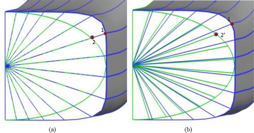
Figure 26. Comparison of wall pressure distributions for the target and final geometry with streamline-based grid along the wall streamlines
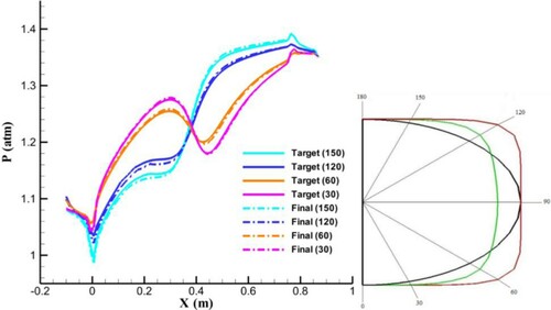
Figure 27. Results of inverse design with different cross-sectional profiles for the initial guess (n = 4) and target geometry (n = 2) using the streamline-based grid and horizontal spines after 200 corrections.
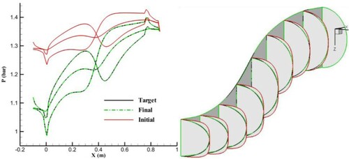
Table 2. Conditions for convergence and unique solution for the inverse design of the s-shape diffuser.
Figure 28. Optimum pressure distribution along the upper and lower lines of the symmetry plane of an S-duct as a TPD for quasi-3D inverse design.
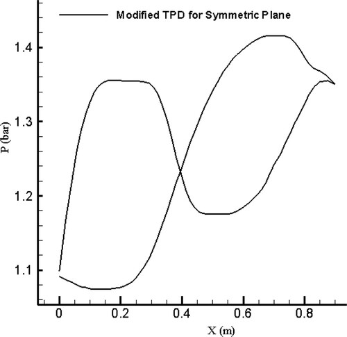
Figure 29. Symmetric plane of the quasi-3D designed S-duct corresponding to the optimum pressure distribution.
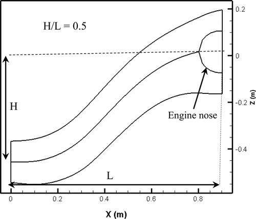
Figure 30. Streamlines through the symmetry plane of the quasi-3D designed S-duct.
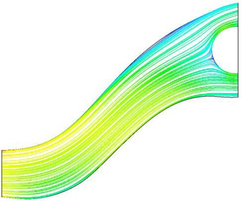
Figure 31. 3D streamlines on the upper wall of the quasi-3D designed S-duct.
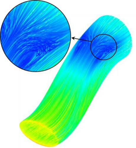
Figure 32. Streamlines and flow separation corresponding to the plane adjacent to the symmetry plane (section D) for the quasi-3D designed S-duct.
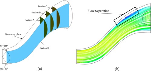
Figure 33. Modification of the wall pressure distribution along the cross sections.
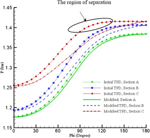
Figure 34. Modified pressure distribution of the upper and lower lines of section D.
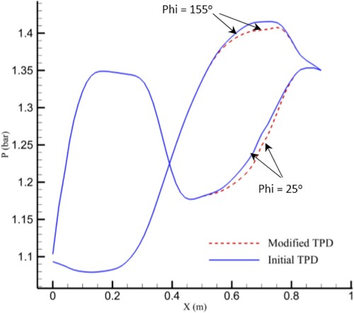
Figure 35. Comparison of the quasi-3D design with the 3D designed S-duct.
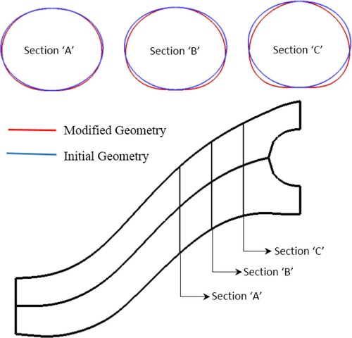
Figure 36. 2D streamlines of section D (a) and 3D streamlines (b) inside the 3D designed S-duct.
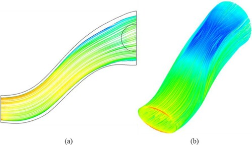
Figure 37. Mach number contours at the outlet of the quasi-3D and 3D designed S-ducts.
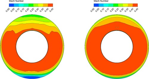
Figure 38. Contours of stagnation pressure in various axial positions for the quasi-3D and 3D designed S-ducts.
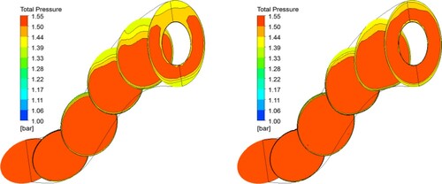
Table 3. Comparison between quasi-3D designed S-duct performance and 3D designed.