Nonlinear conjugate gradient method for identifying Young's modulus of the elasticity imaging inverse problem

Figures & data

Figure 1. Exact and reconstructed ${\mathcal{E}}^k$ (left) and residual error of the coefficient (right) for Example 7.1 at $\eta =0.5\mathrm{\%}$ and $\mathcal{N}\mathcal{E}=\mathrm{20,000}$. The relative error $e_{\mathcal{E}}=0.023$ at k = 30.

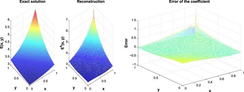
Figure 2. The variation of accuracy error (right) and residual error (left) corresponding to k for Example 7.1.

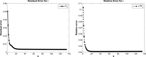
Table 1. The effect of the noise level on the identification parameter for Example 7.1.

$\mathcal{N}\mathcal{E}$	η (%)	k	$e_{\mathcal{E}}$	$\mathcal{J}$	$\mathcal{N}\mathcal{E}$	η (%)	k	$e_{\mathcal{E}}$	$\mathcal{J}$
1800	0.25	45	0.031	0.072	1800	1.50	6	0.049	0.183
1800	0.50	30	0.032	0.074	1800	1.75	5	0.054	0.24
1800	0.75	35	0.0355	0.097	1800	2.00	11	0.059	0.32
1800	1.00	16	0.0397	0.12	1800	2.25	5	0.065	0.47
1800	1.25	12	0.044	0.145	1800	2.50	10	0.071	0.70

Table 2. The numerical results (accuracy error) for Example 7.2.

k	$e_{\mathcal{E}}$	$\mathcal{J}$	k	$e_{\mathcal{E}}$	$\mathcal{J}$
1	0.111373	11.119523	38	0.023302	0.053117
5	0.053033	1.713813	64	0.021767	0.047584
10	0.032814	0.201715	107	0.020590	0.043443
25	0.025083	0.062509	202	0.019473	0.040174

Figure 3. Measurement data at different η, where (a) $\eta =5\mathrm{\%}$, (b) $\eta =1\mathrm{\%}$, and (c) $\eta =0.05\mathrm{\%}$ for Example 7.1.

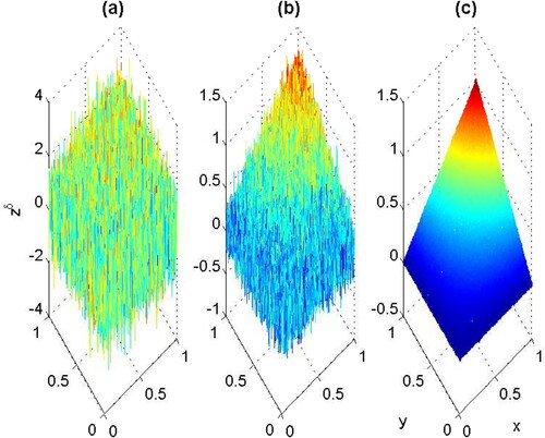
Figure 4. Exact and reconstruction ${\mathcal{E}}^k$ (left), residual error (right) at $k=34$ for Example 7.2, the relative error $e_{\mathcal{E}}=0.0128$ and $\mathcal{J}=0.000521$.

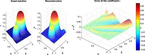
Figure 5. The variation of accuracy error (right) and residual error (left) corresponding to k for Example 7.2.

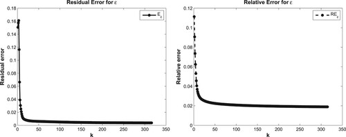
Figure 6. The convergence with $L^2$-gradient corresponding to k for Example 7.2.

Figure 7. A comparison of the residual error E using the present MOLS compared to that of Jadamba et al. [10] and the existing OLS at different starting points ${\mathcal{E}}^0$ for Example 7.3.

Table 3. Performance of the MOLS with increasing $\mathcal{N}\mathcal{E}$ for Example 7.3.

$\mathcal{N}\mathcal{E}$	k	$e_{\mathcal{E}}$	E	Elapsed time (s)
800	31	0.057595	0.057036	599
3200	89	0.043519	0.042320	6050
7200	68	0.039268	0.037950	16,304
12,800	67	0.038095	0.036702	53,964

Jadamba B, Khan A, Rus G, et al. A new convex inversion framework for parameter identification in saddle point problems with an application to the elasticity imaging inverse problem of predicting tumor location. SIAM J Appl Math. 2014;74(5):1486–1510.

 Google Scholar