Force-based stiffness mapping for early detection of breast cancer

Figures & data

Figure 1. Typical 1.95–2.05 g tumours before placement in a phantom.

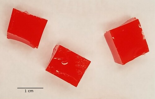
Figure 2. Top view of phantom Tumour B showing tumour location. (The restraining ring has a 110-mm inner diameter.)

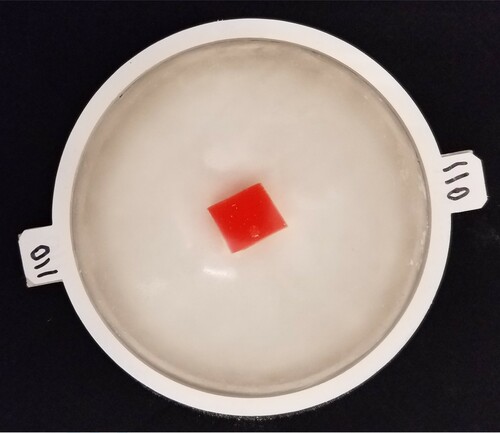
Figure 3. Arc device used to indent the surface of the phantom and record associated forces. (Near the centre of the photo, a white phantom sits in a white tray on the black turntable. Black arches support the indenter mechanism, shown at the $\varphi =10$ degree angle. The rod connects the indenter mechanism through the yellow force sensor to the black indenter head.)

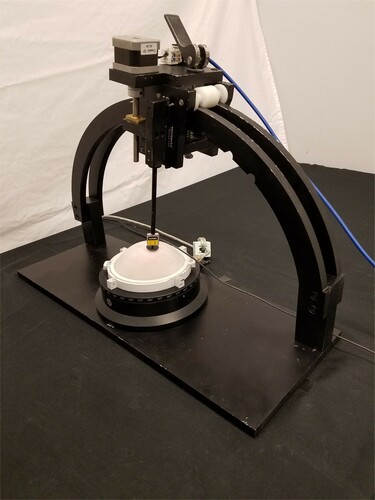
Figure 4. Schematic of indenter head geometry.

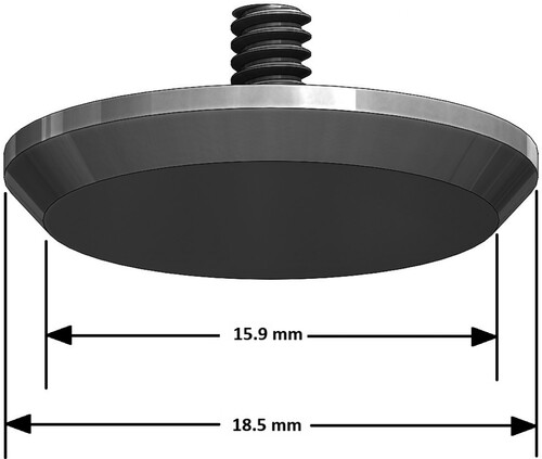
Figure 5. Top view of phantom showing indenter locations. (ϕ is the angle the indenter makes with the vertical and θ is the azimuthal angle. This figure is drawn to scale.)

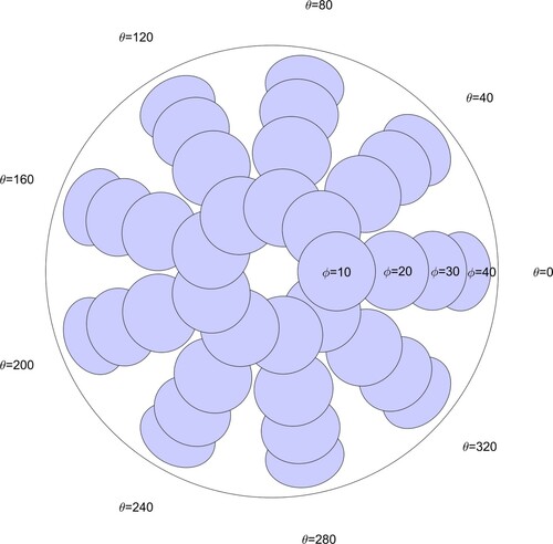
Figure 6. Orientation of scanner used to capture phantom geometry for finite element modelling (left, on arm near laptop) and Arc with phantom (right side) during testing.

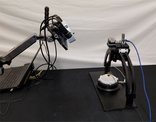
Figure 7. Typical phantom-specific finite element mesh generated from the geometry captured by the scanner. (40 K nodes and 25 K elements.)

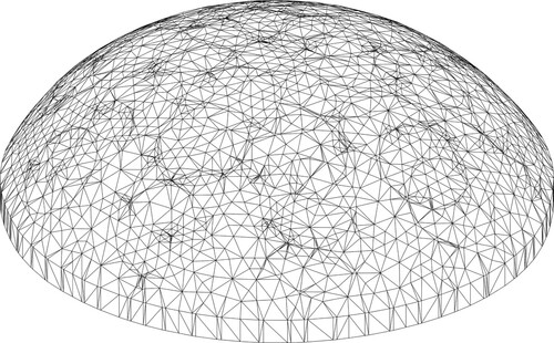
Figure 8. Chromosome used to encode material property information for each individual ($E_h$ is healthy modulus, $E_c$ is cancerous modulus.) [8].

Figure 9. Schematic of phantom side view showing approximate vertical locations of the tumours in the four tumour-containing phantoms.

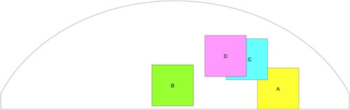
Figure 10. Schematic of phantom top view showing approximate radial locations of the tumours in the tests of the four tumour-containing phantoms. (‘*’ denotes the location of the indenter centres).

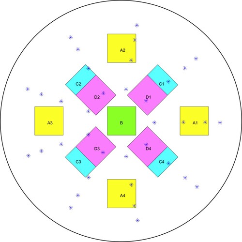
Figure 11. Predicted and true results for Tumour C, test 4. (‘*’ denotes the location of the indenter centres. Note that the vertical line in the middle of the tumour in (d) is the corner of the cube.)

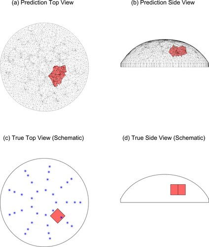
Figure 12. Predicted and true results for Tumour C, test 1. (‘*’ denotes the location of the indenter centres. Note that the vertical line in the middle of the tumour in (d) is the corner of the cube.)

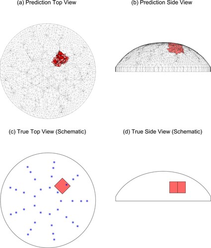
Figure 13. Correct identification of tests at w = 2.0 occurs for 15/16 tumour-free samples and 16/16 tumour-containing samples. (Blue lines indicate range of w for correct identification of tumour-free samples. Red lines indicate range of w for correct identification of tumour-containing samples. Horizontal axis indicates w value, vertical axis gives test name.)

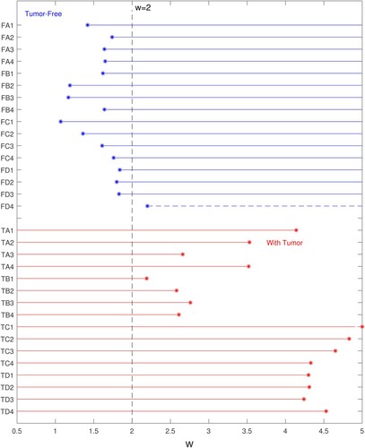
Figure 14. $w_{cross}$ for a given test indicates the strength of the classification. (Horizontal axis indicates $w_{cross}$ value, vertical axis gives test name.)

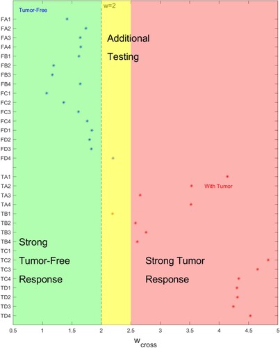
Figure 15. Errors for tumour-free model are small for tumour-free phantoms and high for tumour-containing phantoms. (Horizontal axis gives the error ($1-C{C}_{TF}$), vertical axis gives test name.)

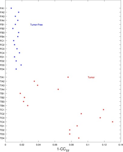
Figure 16. Measured forces for a tumour-free phantom test (FC1) (There are 9 azimuthal test sites at $\theta =0,40,\dots 320$ degrees for each of the elevation angles ϕ.)

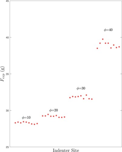
Figure 17. Measured forces (red *- symbols) and tumour-free finite element model results (blue o symbols) for three tests: (a) a tumour-free test (FC1), (b) a test with an easily identified tumour (TC1), and (c) the most difficult-to-identify deep centre tumour (TB1). (Forces are normalized to zero mean. There are 9 azimuthal test sites at $\theta =0,40,\dots 320$ degrees for each of the elevation angles ϕ.)

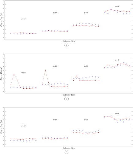
Figure A1. Typical STL geometry produced by scanning the phantom and tray.

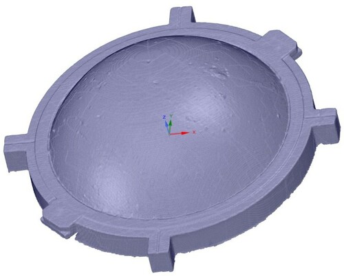
Figure A2. Typical solid geometry for the phantom.

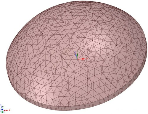
Figure A3. RMS force errors are small for all meshes considered.

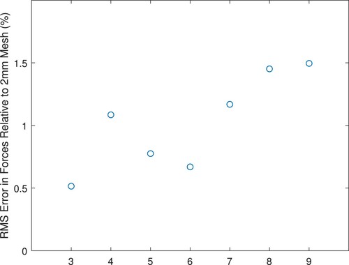
Table B1. Mesh statistics for convergence study (‘Characteristic Elem’ is the characteristic element length reported by ANSYS).

Max Elem	Characteristic Elem (mm)							Serial
Size (mm)	Min	Max	Ave	Std Dev	Nodes	Elements	DOF	Run Time (s)
9	0.04	8.9	2.0	1.5	25456	15009	71400	90
8	0.03	8.1	2.1	1.5	26319	15637	73737	97
7	0.03	7.0	2.1	1.5	27874	16751	77958	129
6	0.04	5.8	2.2	1.1	30861	18888	86367	170
5	0.04	5.2	2.2	1.1	39514	24638	111129	264
4	0.04	3.9	2.1	0.8	59580	38279	166713	648
3	0.04	3.0	1.8	0.5	104499	70566	295611	2293
2	0.04	2.0	1.3	0.2	298799	210492	859644	20241

Figure A4. A typical set of stress–strain data for the 10 tests of a single sample. Notice that a linear elastic material model appears reasonable for this strain range and that the slope of the data ($E_{apparent}$) is similar for all 10 tests.

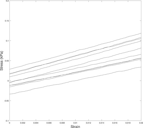
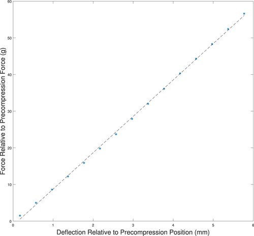
Figure A5. Force–deflection curves for indentation of a tumour-free phantom showing linear behaviour for significant indentation depths. The force is measured relative to a 12 g precompression, and the indentation depth is relative to the depth at 12 g of force. (‘*’ measured data; ‘–’ linear fit to measured data.)

Olson LG, Throne RD, Nolte AJ, et al. An inverse problem approach to stiffness mapping for early detection of breast cancer: tissue phantom experiments. Inverse Probl Sci Eng. 2019;27(7):1006–1037.

 Google Scholar