
Figures & data
Figure 1. High-frequency oscillations during the reconstruction without a general regularization, the example from [Citation13].
![Figure 1. High-frequency oscillations during the reconstruction without a general regularization, the example from [Citation13].](/cms/asset/fc8351a9-d42d-4ce7-853c-b36d2b23ffef/gipe_a_1948025_f0001_oc.jpg)
Figure 2. Low-frequency oscillations during the reconstruction with a general regularization, the example from [Citation13].
![Figure 2. Low-frequency oscillations during the reconstruction with a general regularization, the example from [Citation13].](/cms/asset/473a02b6-e510-411b-8835-11ab6a89879a/gipe_a_1948025_f0002_oc.jpg)
Table 1. The determination of the parent element of the invariant family: item 10 – the parent element , item 16 – the element
with the minimum shift measure
= 0.005315,
= −0.10056.
Figure 3. The observations [Citation35] and the model-calculated population with constant parameters: 1 – the sample , 2 – the direct problem solution
, 3 – the inflection area of the sample, 4 – the inflection point of the solution
.
![Figure 3. The observations [Citation35] and the model-calculated population with constant parameters: 1 – the sample {yi(δ)}i=1,11¯, 2 – the direct problem solution y|a0,1,2(1)=const, 3 – the inflection area of the sample, 4 – the inflection point of the solution y|a0,1,2(1).](/cms/asset/b79ef4f8-89ee-4c1c-9f43-07ad857b5599/gipe_a_1948025_f0003_oc.jpg)
Figure 4. Processing of the observations by smoothing spline: 1 – the population, 2 – the growth rate of the population, 3 – the inflection points of the population.
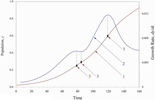
Figure 5. The reconstruction: 1– by the locally sequential refinement,
= 0.004469; 2–
by the formula (18),
= 0.00937;
= 33.0.
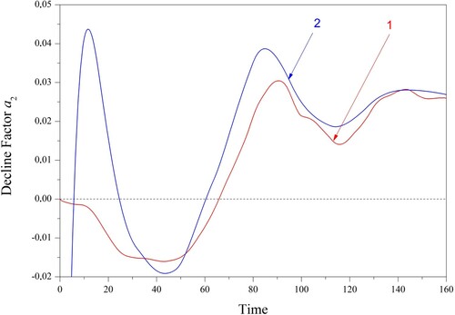
Table 2. The solutions to the inverse problems (13) – (16) for the different α1 and the allocation of the parent element: item 7 – the minimum of the stabilizer, item 10 – the parent element.
Figure 6. The total coronavirus cases in Germany, the source [Citation59]: 1 – the sample , 2 – the spline approximation,
.
![Figure 6. The total coronavirus cases in Germany, the source [Citation59]: 1 – the sample y(δ), 2 – the spline approximation, y~.](/cms/asset/dfafabd9-b92a-47bc-a176-a2738daf44cc/gipe_a_1948025_f0006_oc.jpg)
Figure 7. The spline approximation of the growth rate, , the period of the renewal and decline cycle,
= 6.98 days.
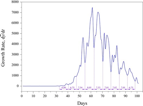
Figure 8. The parameter determined by the formula (18): (a) the initial period, (b) the attenuation period .
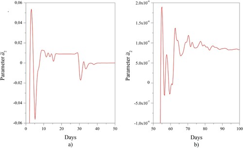
Figure 9. The parameter reconstruction: (a) the general regularization (5) without the locally sequential refinement, (b) the general regularization (5) together with the locally sequential refinement, (c) the used approximation scheme.
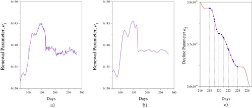
Figure 10. The patterns of the COVID-19 spread in Germany (the symbols mark the moments of the dynamics changes).
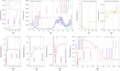
Figure 11. The reconstruction into the large consistency corridor, the worst residuals with observations: ,
,
,
.
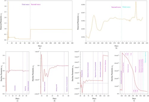
Figure 12. The parameters reconstruction for the different countries, the source of the COVID-19 cases [Citation59]: (a) Sweden; (b) Switzerland; (c) Brazil.
![Figure 12. The parameters reconstruction for the different countries, the source of the COVID-19 cases [Citation59]: (a) Sweden; (b) Switzerland; (c) Brazil.](/cms/asset/202382b6-307f-4914-8054-0be0dfa7d976/gipe_a_1948025_f0012_oc.jpg)