Search in:

Inverse Problems in Science and Engineering Volume 29, 2021 - Issue 13

Submit an article Journal homepage

Free access

662

Views

CrossRef citations to date

Altmetric

Research Article

Sequential estimation of the time-dependent heat transfer coefficient using the method of fundamental solutions and particle filters

W. B. da Silvaa Federal University of Espí-rito Santo, Vitória, BrazilCorrespondence[email protected]

https://orcid.org/0000-0003-2242-7825 View further author information

J. C. S. Dutraa Federal University of Espí-rito Santo, Vitória, Brazil

https://orcid.org/0000-0001-6784-4150 View further author information

C. E. P. Kopperschimidta Federal University of Espí-rito Santo, Vitória, BrazilView further author information

D. Lesnicb Department of Applied Mathematics, University of Leeds, Leeds, UKView further author information

R. G. Aykroydc Department of Statistics, University of Leeds, Leeds, UK

https://orcid.org/0000-0003-3700-0816 View further author information

Pages 3322-3341 | Received 21 Nov 2019, Accepted 17 Oct 2021, Published online: 07 Nov 2021

Cite this article
https://doi.org/10.1080/17415977.2021.1998040
CrossMark

Full Article
Figures & data
References
Citations
Metrics
Reprints & Permissions
View PDF PDF View EPUB EPUB

Figures & data

Figure 1. The analytical and MFS numerical solutions for: (a) $T (x, 0.5)$ , (b) $T (1, t)$ , (c) $T (0, t)$ and (d) $E (t)$ , obtained when solving the direct problem for Example 1. Corresponding to the results for $T (x, 0.5)$ , $T (1, t)$ , $T (0, t)$ and $E (t)$ , the maximum pointwise relative errors between the analytical and numerical MFS solutions are $0.5 %$ , $0.2 %$ , $0.3 %$ and $0.01 %$ , respectively.

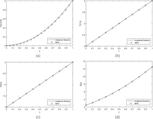
Figure 2. Estimated $ρ (t)$ and the filtered boundary temperature measurements (Equation19(19) $\begin{aligned} Y_{a} (t_{k}) = Y (t_{k}) + ϵ_{k}, k = 1, \dots, M, \end{aligned}$ (19) ) contaminated with $p = 1 %$ noise, obtained using the particle filter with $N_{part} = 200$ particles for (a) and (c) $σ_{ρ} = 0.2$ ; (b) and (d) $σ_{ρ} = 0.4$ , for Example 1.

Figure 2. Estimated ρ(t) and the filtered boundary temperature measurements (Equation19(19) Ya(tk)=Y(tk)+ϵk,k=1,…,M,(19) ) contaminated with p=1% noise, obtained using the particle filter with Npart=200 particles for (a) and (c) σρ=0.2; (b) and (d) σρ=0.4, for Example 1.

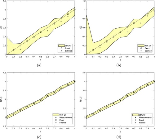
Table 1. Results for various $σ_{ρ}$ for $p = 1 %$ noise in Equation (Equation19(19) $\begin{aligned} Y_{a} (t_{k}) = Y (t_{k}) + ϵ_{k}, k = 1, \dots, M, \end{aligned}$ (19) ) for Example 1.

Display Table

Table 2. Results for $p = 5 %$ noise in Equation (Equation19(19) $\begin{aligned} Y_{a} (t_{k}) = Y (t_{k}) + ϵ_{k}, k = 1, \dots, M, \end{aligned}$ (19) ) with $σ_{ρ} = 0.2$ for Example 1.

Display Table

Table 3. Results for $p \in {1, 5} %$ noise in Equation (Equation20(20) $\begin{aligned} E_{a} (t_{k}) = E (t_{k}) + ϵ_{k}, k = 1, \dots, M, \end{aligned}$ (20) ) with $σ_{ρ} = 0.2$ for Example 1.

Display Table

Figure 3. Estimated $ρ (t)$ and the filtered measurements (Equation20(20) $\begin{aligned} E_{a} (t_{k}) = E (t_{k}) + ϵ_{k}, k = 1, \dots, M, \end{aligned}$ (20) ) contaminated with $p = 1 %$ noise, obtained using the particle filter with $σ_{ρ} = 0.2$ and $N_{part} = 200$ particles, for Example 1.

Figure 3. Estimated ρ(t) and the filtered measurements (Equation20(20) Ea(tk)=E(tk)+ϵk,k=1,…,M,(20) ) contaminated with p=1% noise, obtained using the particle filter with σρ=0.2 and Npart=200 particles, for Example 1.

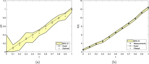
Figure 4. Estimated $ρ (t)$ from the measurements (a) (Equation19(19) $\begin{aligned} Y_{a} (t_{k}) = Y (t_{k}) + ϵ_{k}, k = 1, \dots, M, \end{aligned}$ (19) ) or (b) (Equation20(20) $\begin{aligned} E_{a} (t_{k}) = E (t_{k}) + ϵ_{k}, k = 1, \dots, M, \end{aligned}$ (20) ) contaminated with $p = 5 %$ noise, as filtered in (c) and (d), respectively, obtained using the particle filter with $σ_{ρ} = 0.2$ and $N_{part} = 200$ particles, for Example 1.

Figure 4. Estimated ρ(t) from the measurements (a) (Equation19(19) Ya(tk)=Y(tk)+ϵk,k=1,…,M,(19) ) or (b) (Equation20(20) Ea(tk)=E(tk)+ϵk,k=1,…,M,(20) ) contaminated with p=5% noise, as filtered in (c) and (d), respectively, obtained using the particle filter with σρ=0.2 and Npart=200 particles, for Example 1.

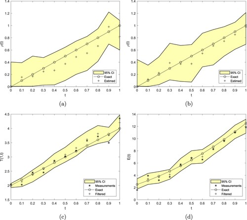
Figure 5. The variation of the MWCI over time for (a) $p = 1 %$ and (b) $p = 5 %$ noise in Equation (Equation19(19) $\begin{aligned} Y_{a} (t_{k}) = Y (t_{k}) + ϵ_{k}, k = 1, \dots, M, \end{aligned}$ (19) ) or Equation (Equation20(20) $\begin{aligned} E_{a} (t_{k}) = E (t_{k}) + ϵ_{k}, k = 1, \dots, M, \end{aligned}$ (20) ), obtained using the particle filter with $σ_{ρ} = 0.2$ and $N_{part} = 200$ particles, for Example 1.

Figure 5. The variation of the MWCI over time for (a) p=1% and (b) p=5% noise in Equation (Equation19(19) Ya(tk)=Y(tk)+ϵk,k=1,…,M,(19) ) or Equation (Equation20(20) Ea(tk)=E(tk)+ϵk,k=1,…,M,(20) ), obtained using the particle filter with σρ=0.2 and Npart=200 particles, for Example 1.

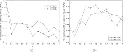
Figure 6. The analytical and MFS numerical solutions for: (a) $T (1, t)$ , (b) $T (0, t)$ , (c) $E (t)$ , obtained when solving the direct problem for Example 2. Corresponding to the results for $T (1, t)$ , $T (0, t)$ and $E (t)$ , the maximum pointwise relative errors between the analytical and numerical MFS solutions are $4 %$ , $2 %$ and $0.2 %$ , respectively.

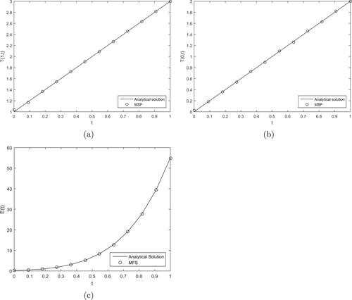
Figure 7. (a) Estimated $ρ (t)$ from the measurements (Equation20(20) $\begin{aligned} E_{a} (t_{k}) = E (t_{k}) + ϵ_{k}, k = 1, \dots, M, \end{aligned}$ (20) ) with (a) $p = 1 %$ and (b) $p = 5 %$ noise, as filtered in (c) and (d), respectively, along with (e) the variation of the MWCI over time, obtained using the particle filter with $σ_{ρ} = 0.2$ and $N_{part} = 200$ particles, for Example 2.

Figure 7. (a) Estimated ρ(t) from the measurements (Equation20(20) Ea(tk)=E(tk)+ϵk,k=1,…,M,(20) ) with (a) p=1% and (b) p=5% noise, as filtered in (c) and (d), respectively, along with (e) the variation of the MWCI over time, obtained using the particle filter with σρ=0.2 and Npart=200 particles, for Example 2.

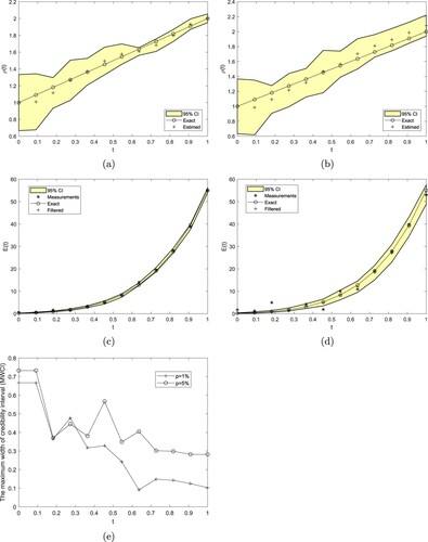
Table 4. Results for $p \in {1, 5} %$ noise in Equation (Equation20(20) $\begin{aligned} E_{a} (t_{k}) = E (t_{k}) + ϵ_{k}, k = 1, \dots, M, \end{aligned}$ (20) ) with $σ_{ρ} = 0.2$ for Example 2.

Display Table

Reprints and Corporate Permissions

Please note: Selecting permissions does not provide access to the full text of the article, please see our help page How do I view content?

To request a reprint or corporate permissions for this article, please click on the relevant link below:

Order Reprints Request Corporate Permissions

Academic Permissions

Please note: Selecting permissions does not provide access to the full text of the article, please see our help page How do I view content?

Obtain permissions instantly via Rightslink by clicking on the button below:

Request Academic Permissions

If you are unable to obtain permissions via Rightslink, please complete and submit this Permissions form. For more information, please visit our Permissions help page.

Share icon
Back to Top

Related research

People also read lists articles that other readers of this article have read.

Recommended articles lists articles that we recommend and is powered by our AI driven recommendation engine.

Cited by lists all citing articles based on Crossref citations.
Articles with the Crossref icon will open in a new tab.

People also read
Recommended articles
Cited by

To cite this article:

Reference style: APA Chicago Harvard

Citation copied to clipboard

Reference styles above use APA (6th edition), Chicago (16th edition) & Harvard (10th edition)

Download citation

Download a citation file in RIS format that can be imported by citation management software including EndNote, ProCite, RefWorks and Reference Manager.

Choose format: RIS BibTex RefWorks Direct Export

Choose options: Citation Citation & abstract Citation & references

Sequential estimation of the time-dependent heat transfer coefficient using the method of fundamental solutions and particle filters

Table 1. Results for various $σ_{ρ}$ for $p = 1 %$ noise in Equation (Equation19(19) $\begin{aligned} Y_{a} (t_{k}) = Y (t_{k}) + ϵ_{k}, k = 1, \dots, M, \end{aligned}$ (19) ) for Example 1.

Table 2. Results for $p = 5 %$ noise in Equation (Equation19(19) $\begin{aligned} Y_{a} (t_{k}) = Y (t_{k}) + ϵ_{k}, k = 1, \dots, M, \end{aligned}$ (19) ) with $σ_{ρ} = 0.2$ for Example 1.

Table 3. Results for $p \in {1, 5} %$ noise in Equation (Equation20(20) $\begin{aligned} E_{a} (t_{k}) = E (t_{k}) + ϵ_{k}, k = 1, \dots, M, \end{aligned}$ (20) ) with $σ_{ρ} = 0.2$ for Example 1.

Table 4. Results for $p \in {1, 5} %$ noise in Equation (Equation20(20) $\begin{aligned} E_{a} (t_{k}) = E (t_{k}) + ϵ_{k}, k = 1, \dots, M, \end{aligned}$ (20) ) with $σ_{ρ} = 0.2$ for Example 2.

Information for

Open access

Opportunities

Help and information

Your download is now in progress and you may close this window

Login or register to access this feature

Sequential estimation of the time-dependent heat transfer coefficient using the method of fundamental solutions and particle filters

Figures & data

Table 1. Results for various σρ for p=1% noise in Equation (Equation19(19) Ya(tk)=Y(tk)+ϵk,k=1,…,M,(19) ) for Example 1.

Table 2. Results for p=5% noise in Equation (Equation19(19) Ya(tk)=Y(tk)+ϵk,k=1,…,M,(19) ) with σρ=0.2 for Example 1.

Table 3. Results for p∈{1,5}% noise in Equation (Equation20(20) Ea(tk)=E(tk)+ϵk,k=1,…,M,(20) ) with σρ=0.2 for Example 1.

Table 4. Results for p∈{1,5}% noise in Equation (Equation20(20) Ea(tk)=E(tk)+ϵk,k=1,…,M,(20) ) with σρ=0.2 for Example 2.

Reprints and Corporate Permissions

Academic Permissions

Related research

To cite this article:

Download citation

Information for

Open access

Opportunities

Help and information

Keep up to date

Table 1. Results for various $σ_{ρ}$ for $p = 1 %$ noise in Equation (Equation19(19) $\begin{aligned} Y_{a} (t_{k}) = Y (t_{k}) + ϵ_{k}, k = 1, \dots, M, \end{aligned}$ (19) ) for Example 1.

Table 2. Results for $p = 5 %$ noise in Equation (Equation19(19) $\begin{aligned} Y_{a} (t_{k}) = Y (t_{k}) + ϵ_{k}, k = 1, \dots, M, \end{aligned}$ (19) ) with $σ_{ρ} = 0.2$ for Example 1.

Table 3. Results for $p \in {1, 5} %$ noise in Equation (Equation20(20) $\begin{aligned} E_{a} (t_{k}) = E (t_{k}) + ϵ_{k}, k = 1, \dots, M, \end{aligned}$ (20) ) with $σ_{ρ} = 0.2$ for Example 1.

Table 4. Results for $p \in {1, 5} %$ noise in Equation (Equation20(20) $\begin{aligned} E_{a} (t_{k}) = E (t_{k}) + ϵ_{k}, k = 1, \dots, M, \end{aligned}$ (20) ) with $σ_{ρ} = 0.2$ for Example 2.