Identification of airborne pollutant sources within a slot ventilated porous enclosure depending on backward model and downwind scheme

Figures & data

Figure 1. Flow configuration and coordinate system.

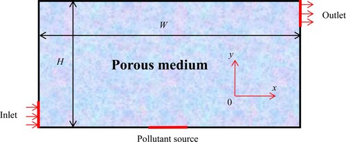
Table 1. Grid independence validation: Sh number for different grid resolution.

Grid sizes	41×81	61×121	101×201	121×241
Sh	17.63	24.30	26.26	26.73

Figure 2. A schematic diagram of the flow through two parallel-plate channel partially filled with two porous substrates.

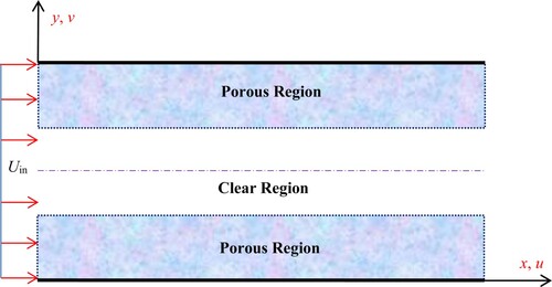
Figure 3. Flow chart of direct CFD procedure simulation algorithm.

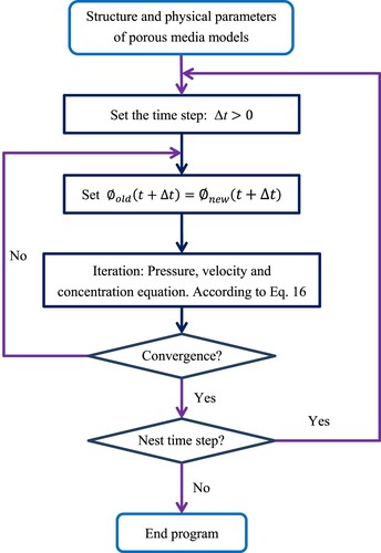
Figure 4. A comparison of the present work fully developed axial velocity with the solution given by Alkam et al. [33] for $Da=1\times {10}^{-4}$.

Figure 5. Comparison of the velocity and temperature profiles between the present prediction and Khanafer and Chamkha [34].

Figure 6. Flow chart of inverse time simulation algorithm.

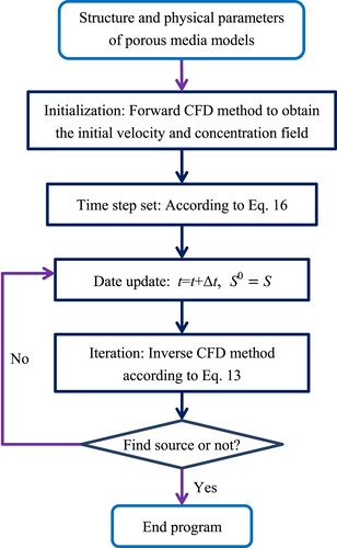
Figure 7. Streamlines (left) and pollutant concentration fields (right) with Re=1.0×10³, Sc=0.6 at t=100.

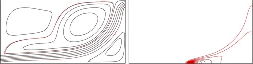
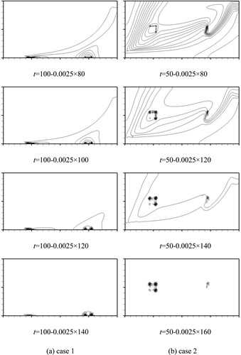
Figure 8. The inverse results of pollutant source location, Q-R (left) and new study (right).

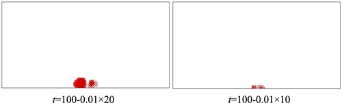
Figure 9. Streamlines (left) and pollutant concentration fields (right) with Re=2×10³, Sc=0.8, Da=2.5×10⁻³ at t=150

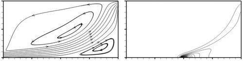
Figure 10. Effect of temporal step size on backward simulation with Re=2×10³, Sc=0.8 and Da=2.5×10⁻³, (a) Δt=−0.025, (b) Δt=−0.05, and (c) Δt=−0.1

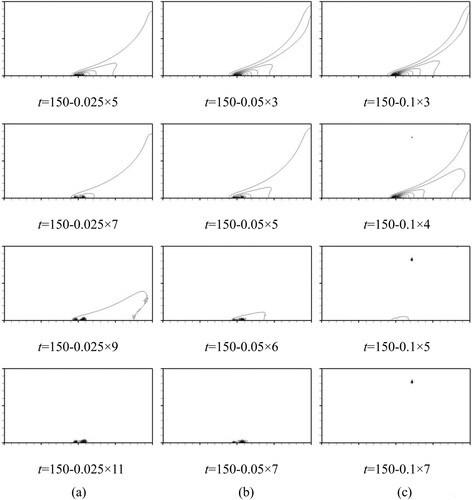
Figure 11. Streamlines (left) and pollutant concentration fields (right) with Sc=0.8, Da=5×10⁻⁴ at t=100, (a) Re=2×10², (b) Re=2×10³, and (c) Re=1×10⁴

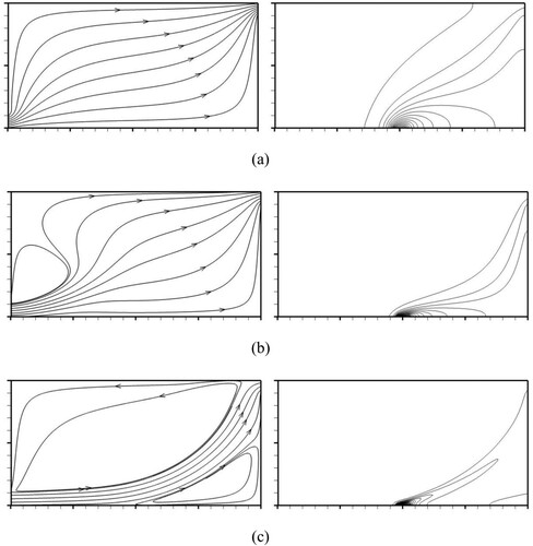
Figure 12. Effect of Re on backward simulation with Sc=0.8 and Da=5×10⁻⁴, (a) Re=2×10², (b) Re=2×10³, and (c) Re=1×10⁴

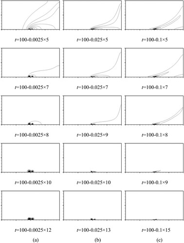
Figure 13 Streamlines and backward simulations with Re=2×10³, Sc=0.8, (a) Da=5×10⁻⁵, (b) Da=5×10⁻⁴, and (c) Da=5×10⁻³.

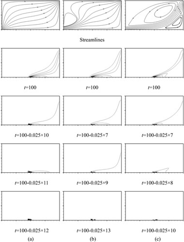
Figure 14. Effect of Sc on backward simulation with Re=2×10³ and Da=2.5×10⁻³, (a) Sc=0.1, (b) Sc=0.8, and (c) Sc=2.0.

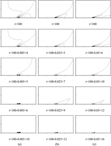
Figure 15. Effect of pollutant sources on backward simulation with Re=2×10³, Da=2.5×10⁻³, Sc=0.8 and Δt=−0.025.

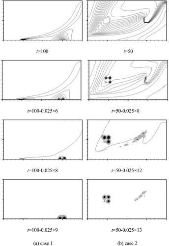
Figure 16. Effect of pollutant sources on backward simulation with Re=2×10³, Da=2.5×10⁻³, Sc=0.8 and Δt=−0.0025

Alkam MK, Al-Nimr MA, Hamdan MO. On forced convection in channels partially filled with porous substrates. Heat Mass Transf. 2002;38(4-5):337–342. DOI:10.1007/s002310000177

 Web of Science ®Google Scholar

Khanafer KM, Chamkha AJ. Mixed convection flow in a lid-driven enclosure filled with a fluid-saturated porous medium. Int J Heat Mass Transfer. 1999;42(13):2465–2481. DOI:10.1016/S0017-9310(98)00227-0

 Web of Science ®Google Scholar