A New Approach to Analytical Modeling of Mars’s Magnetic Field

Figures & data

Figure 1. Isoline maps of the total magnetic field B at an altitude of 150 km according to the source model data [14] obtained by (a) transformation using spherical harmonics and (b) solution of the inverse problem using modified S-approximations; (c) heat map of value differences between source model data and the result of S-approximations; (d) frequency histogram of value differences between (a) and (b).

Figure 2. Isoline maps of the total magnetic field B at an altitude of 120 km according to the source model data [14] obtained by (a) transformation using spherical harmonics and (b) analytic downward continuations within modified S-approximations; (c) heat map of value differences between (a) and (b); (d) frequency histogram of value differences between (a) and (b).

Figure 3. Isoline maps of the total magnetic field B at an altitude of 90 km according to the source model data [14] obtained by (a) transformation using spherical harmonics and (b) analytic downward continuations within modified S-approximations; (c) heat map of value differences between (a) and (b); (d) frequency histogram of value differences between (a) and (b).

Figure 4. Isoline maps of the total magnetic field B at an altitude of 60 km according to the source model data [14] obtained by (a) transformation using spherical harmonics and (b) analytic downward continuations within modified S-approximations; (c) heat map of value differences between (a) and (b); (d) frequency histogram of value differences between (a) and (b).

Figure 5. Isoline maps of the total magnetic field B on the surface according to the source model data [14] obtained by (a) transformation using spherical harmonics and (b) analytic downward continuations within modified S-approximations; (c) heat map of value differences between (a) and (b); (d) frequency histogram of value differences between (a) and (b).

Figure 6. Quantitative maps of the distribution of equivalent sources, using modified S-approximations at depths of (a) 1 km, (b) 10 km below the relief.

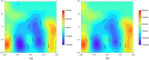
Table 1. Descriptive statistics for data on the total magnetic field at different altitudes according to the spherical harmonics model (L), the model of S-approximations (S), and the difference between them (D).

Altitude-model	Minimum	Maximum	Mean	Median	Root Mean Square	Variance	Standard Deviation	Range
150-L	0,69	256,09	57,35	44,30	78,60	2890,09	53,76	255,40
120-L	1,00	361,08	78,98	58,56	108,95	5631,46	75,04	360,08
90-L	1,85	532,78	113,13	79,40	157,20	11914,14	109,15	530,93
60-L	1,04	860,20	170,46	112,71	239,63	28382,43	168,47	859,16
0-L	2,87	2762,79	454,89	295,65	640,75	203755,76	451,39	2759,93
150-S	0,57	257,23	57,74	44,31	79,35	2963,84	54,44	256,66
120-S	0,82	288,90	60,93	44,64	82,91	3164,05	56,25	288,08
90-S	1,23	377,91	76,15	56,99	69,98	4170,31	64,58	376,68
60-S	4,75	701,46	155,61	122,63	202,31	16726,91	129,33	696,71
0-S	17,56	15163,46	3950,82	2386,19	5373,73	13275910,34	3643,61	15145,90
150-D	−1,14E-06	1,48E-06	2,14E-07	1,93E-07	3,87E-07	1,04E-13	3,23E-07	2,62E-06
120-D	−35,09	111,85	18,04	10,69	29,16	525,04	22,91	146,94
90-D	−126,81	305,02	36,60	17,15	70,11	3576,07	59,80	431,83
60-D	−460,10	621,43	12,96	−6,40	134,86	18021,79	134,25	1081,53
0-D	−15273,44	1017,90	−3547,29	−2739,04	4790,02	10362056,62	3219,01	16291,34

Langlais B, Thébault E, Houliez A, et al. A new model of the crustal magnetic field of Mars using MGS and MAVEN. J. Geophys Res Planet. 2019;124:1542–1569.

 Web of Science ®Google Scholar