A method for determining the parameters in a rheological model for viscoelastic materials by minimizing Tikhonov functionals

Figures & data

Figure 1. Strain–time curve ε with strain rate η and maximum strain value $\overline{ϵ}$.

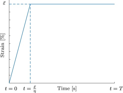
Figure 2. Rheological model with three Maxwell elements.

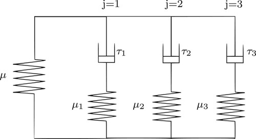
Figure 3. Strain–time curves for different displacement rates ${\eta }_u$.

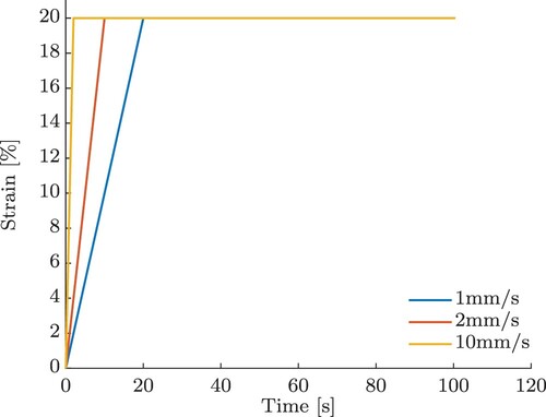
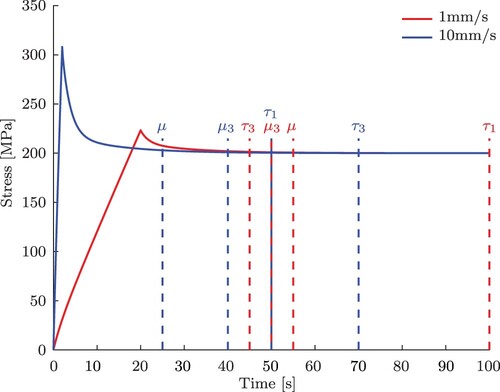
Figure 4. Synthetic stress–time data produced by a model consisting of a spring combined with three Maxwell elements for three different displacement rates.

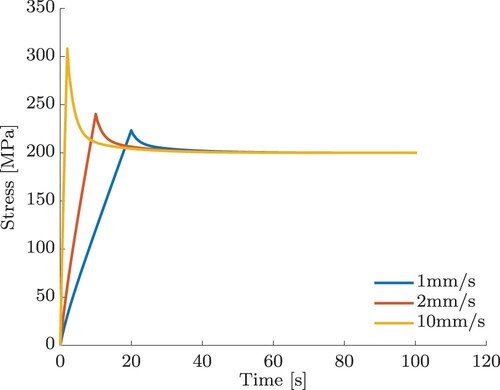
Table 1. Selected material parameters to simulate data.

j	0	1	2	3
${\mu }_j$ [MPa]	10	4	7	1
${\tau }_j$ [s]	–	0.2	3.7	25

Table 2. Reconstructed material parameters before and after clustering where the ${\mu }_j$ are given in MPa and the ${\tau }_j$ in seconds.

$j=$	0	1	2	3	4	5
Reconstructed values
${\mu }_j$	10.000	4.000	3.685	1.621	1.694	1.000
${\tau }_j$	–	0.200	3.695	3.706	3.706	25.000
After clustering
${\mu }_j$	10.000	4.000	7.000	1.000
${\tau }_j$	–	0.200	3.700	25.000

Table 3. Approximated material parameters with similar noisy data, where the ${\mu }_j$ are given in MPa and the ${\tau }_j$ in seconds.

$j=$		0	1	2	3
Exact values	${\mu }_j$	10	4	7	1
	${\tau }_j$	–	0.2	3.7	25
Experiment 1	${\mu }_j$	9.9951	38.558	7.2098	0.88371
	${\tau }_j$	–	0.019903	3.7734	27.795
Experiment 2	${\mu }_j$	10.005	2.475	6.9957	1.0157
	${\tau }_j$	–	0.29222	3.6908	24.2965
Experiment 3	${\mu }_j$	9.99348	44.351	7.2084	0.96407
	${\tau }_j$	–	0.01344	3.6444	26.633
Experiment 4	${\mu }_j$	10.003	7.3458	7.0398	0.99887
	${\tau }_j$	–	0.0993	3.6626	24.0342

Figure 5. Spread of the material parameters $({\mu }_1,{\tau }_1)$ for 100 runs with different noise seeds, but same noise level ${\delta }_{rel}$ for ${\eta }_u$ = 10 mm/s.

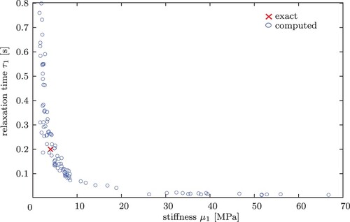
Table 4. Clustered material parameters with noisy data ($\eta =1$ mm/s) where the ${\mu }_j$ are given in MPa and the ${\tau }_j$ in seconds.

$j=$		0	1	2	3
Exact values	${\mu }_j$	10	4	7	1
	${\tau }_j$	–	0.2	3.7	25
Experiment 1	${\mu }_j$	9.9945	27.367	5.945	0.91663
	${\tau }_j$	–	0.088687	4.2318	27.263
Experiment 2	${\mu }_j$	10.007	–	7.5694	1.0434
	${\tau }_j$	–	–	3.4762	23.689
Experiment 3	${\mu }_j$	9.0111	2.6942	7.2928	1.0402
	${\tau }_j$	–	0.82841	6.3049	3000.5
Experiment 4	${\mu }_j$	10.006	2.094	6.0643	1.0303
	${\tau }_j$	–	0.885029	3.9963	23.423

Figure 6. Individual stress components for a displacement rate of 1 mm/s.

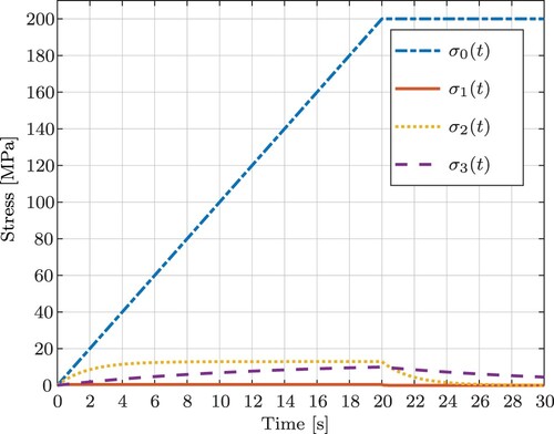
Figure 7. Individual stress components for a displacement rate of 10 mm/s.

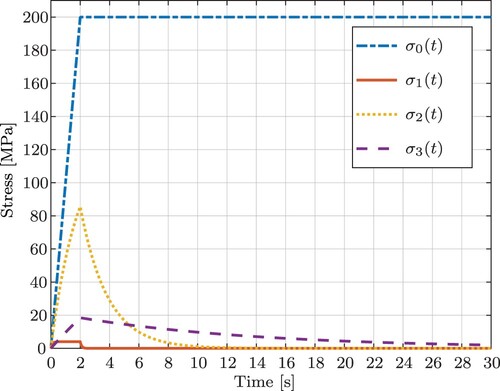
Table 5. Maximum values of individual stress components (MPa) with slow and fast deformation rates attained at $t=\overline{ϵ}/\eta$.

		j = 1	j = 2	j = 3
$\eta =1$	${\sigma }_j\left(\overline{ϵ}/\eta \right)$	0.4	12.94	9.9
$\eta =10$	${\sigma }_j\left(\overline{ϵ}/\eta \right)$	4	85.57	18.48

Table 6. Clustered material parameters with and without regularization where the ${\mu }_j$ are given in MPa and the ${\tau }_j$ in seconds.

$j=$		0	1	2	3
Exact values	${\mu }_j$	10	4	7	1
	${\tau }_j$	–	0.2	3.7	25
Without	${\mu }_j$	10.0003	6.9146	6.9963	0.9909
regularization	${\tau }_j$	–	0.1096	3.7056	25.3752
With	${\mu }_j$	10.0065	4.214	6.9556	1.1312
regularization	${\tau }_j$	–	0.1607	3.5549	22.2532

Figure 8. Smallest relaxation time determined from 100 runs with (a) no regularization, (b) classical Tikhonov–Phillips regularization and (c) adjusted regularization term.

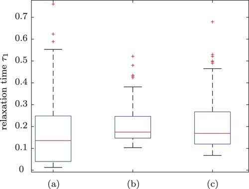
Figure 9. Largest relaxation time for 100 runs with (a) no regularization, (b) classical Tikhonov–Phillips regularization and (c) adjusted regularization term.

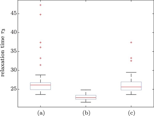
Figure 10. Effect of reducing the duration $[0,T]$ of the experiment on the material parameters $\mu ,{\mu }_3,{\tau }_1$ and ${\tau }_3$ for a displacement rate of 10 mm/s (left) and 1 mm/s (right), respectively.

Figure 11. Synthetic stress–time data produced by a spring combined with a three Maxwell element model including the duration of the experiment to conclusively identify the stiffnesses and relaxation times for displacement rates of 1 mm/s and 10 mm/s.