Figures & data
Figure 1. Hazard evaluation flow chart. Note that time durations and the definition of stability need to be determined by the assessor on a case-specific basis. Example durations are based on typical daily water renewals used in bioassay test methods. “Dispersible” is functionally and conservatively defined as ≥1% of the original concentration. “Stable” is functionally defined as ±20% of the initial concentration (Petersen et al., Citation2015; OECD, Citation2012; Coleman et al., Citation2015, Citation2017a, Citation2017b).
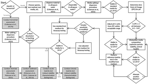
Table 1. Nanoparticle characterization, toxicity test decisions and results for the three case studies. Primary particle size and hydrodynamic diameter (HD) were determined in the stock by ImagePro measurements of transmission electron microscopy images and by dynamic light scattering (DLS), respectively. Data are presented as means (± 1 standard deviation), ranges (min–max) and the number of particles counted (N) are provided. Toxicity endpoints are expressed with 95% confidence ranges in parentheses. Additional data are reported in the Supplementary Material. IS: ionic strength; NA: not available; MHRW: moderately hard reconstituted water.
Figure 2. Pre-test results for Case Study 2 using TiO2. Photospectrometry (λ = 300) was used in initial pretests to quickly generate particle settling curves and indicated that (A) settling rates and (B) agglomeration rates (by dynamic light scattering) in moderately hard reconstituted water (300 μS/cm) were highly concentration dependent. (C) Agglomeration rates were not substantially altered by adjusting pH from 7.8 to 8.7. In diluted 100 μS/cm water (pH8.7), pretests by (D) photospectrometry (λ = 300) and by (E) measured concentrations standardized by the initially measured concentration at time zero (B; see Supplementary Figure S3A actual concentrations) also indicated concentration dependent settling. (F) Agglomeration was reduced but not eliminated compared to ultrapure water even at low conductivity (3 μS/cm) not suitable for C. dubia testing. Dashed horizontal lines in each plot indicate an operational definition of stability (±20% of the initial value).
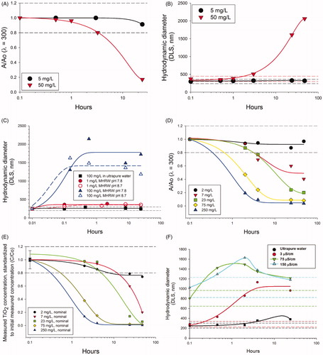
Figure 3. Determination of the impact of adjusting pH on the zeta potential (mV) of nano TiO2.
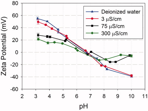
Figure 4. Ceriodaphnia dubia dose response curves for (A) probe sonicated and (B) bath sonicated TiO2. Time-weighted averaged data provided an improved estimate of the actual organism exposure to the settling TiO2 particles during the bioassay. The rapid agglomeration and subsequent settling of the TiO2 in the highest four concentrations reduced organism exposure to the suspended TiO2, and concentration expressed as nominal or mean measured over-represented the actual organism exposure to TiO2.
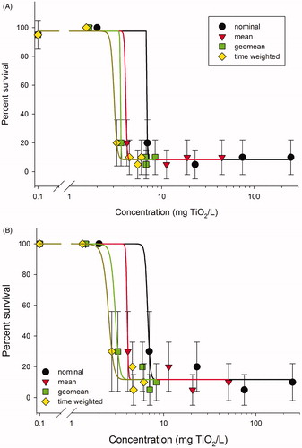
Figure 5. Delayed effects of TiO2 exposure on C. dubia after being exposed continuously or for various time periods, followed by transfer to clean 100 μS/cm water. Circles represent organisms exposed for the indicated durations and then transferred to clean test media. Triangles represent organisms continuously exposed over the 48 h test duration. The non-linear regression (dashed line) is fit to all data from both exposure regimes.
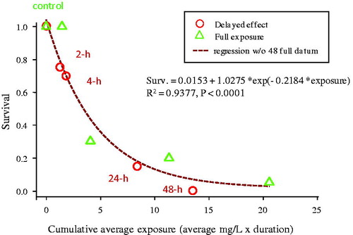
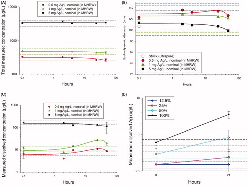
Figure 6. Functional test results for Case Study 3 using PVP-AgNPs. (A) Total measurable silver concentration and (B) hydrodynamic diameter by dynamic light scattering were relatively stable (± 20%) for at least 48 h. (C) However, dissolved concentrations changed by more than ±20% during the 48 h period. (D) The lower concentrations of particles tested in the bioassays resulted in consistent increases in dissolved Ag concentrations; percentages in the legend represent the dilution series with the 100% being the highest concentration. The lowest two PVP-AgNP treatments do not appear in the graph because the dissolved concentrations were below analytical detection limits (<0.5 μg Ag/l μg/l). Dashed lines indicate ±20% of the initial value.