Three-dimensional numerical simulations and proper orthogonal decomposition analysis of flow over different bottom-mounted ribs

Figures & data

Figure 1. Computational domain and boundary conditions: (a) 2D XY-plane and (b) 3D view.

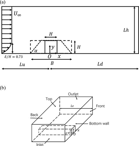
Table 1. Results for all the bottom-mounted ribs based on the mesh elements and the time-step.

Case		No. of cells	Grids in Z direction	Δt	$\overline{C_D}$	$\overline{C_L}$	Lw
	1	1,275,219	33	0.002	1.116	0.567	14.168
	2	1,652,970	33	0.002	1.121	0.572	13.626
Square rib	3	2,140,512	33	0.002	1.133	0.581	12.907
	4	2,140,512	33	0.001	1.132	0.580	12.907
	5	2,140,512	33	0.003	1.131	0.579	12.907
	6	3,113,472	48	0.002	1.133	0.581	13.172
	7	1,275,219	33	0.002	0.806	0.261	13.702
Trapezoidal rib	8	1,652,970	33	0.002	0.825	0.272	12.400
	9	2,140,512	33	0.002	0.844	0.287	10.195
	10	1,275,219	33	0.002	0.961	0.490	18.213
Rectangular rib	11	1,652,970	33	0.002	0.985	0.499	15.812
	12	2,140,512	33	0.002	1.006	0.527	11.755

Figure 2. Profiles of the time- and spanwise-averaged (a) streamwise velocity and (b) pressure at $y/H=0.004$ for Cases 1–6.

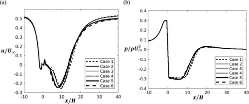
Figure 3. Time- and spanwise-averaged streamwise velocity profiles of Cases 1–6.

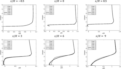
Figure 4. Computational mesh of the square rib (Case 3): (a) full XY-plane domain and (b, c) closer view around the rib.

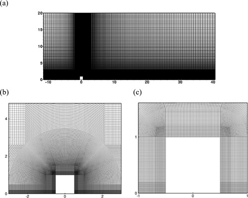
Figure 5. Time-averaged streamwise velocities of Case 3 compared with the experimental data reported by Liu et al. (2008).

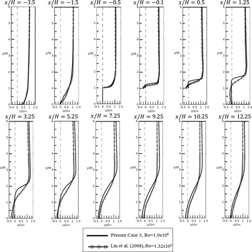
Figure 6. Wall-normal positions of the local maximum time- and spanwise-averaged root-mean-square value of the streamwise velocity fluctuations.

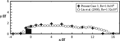
Table 2. Comparison of Case 3 with the numerical results reported by Tauqeer et al. (2017).

Configuration	Author	Flow conditions	$C_D$	$L_w$
Square	Case 3	$Re=1\times {10}^6$, $\delta /H=0.73$	1.133	12.907
	Tauqeer et al. (2017)	$Re=1\times {10}^6$, $\delta /H=0.73$	1.16	12.02

Figure 7. Power spectra of the velocity fluctuations at $y/H=0.5$ with a distance of $0.5H$ to the back face of the ribs for (a) square, (b) trapezoidal and (c) rectangular ribs. The red lines represent the −5/3 law. (This figure is available in colour online.)

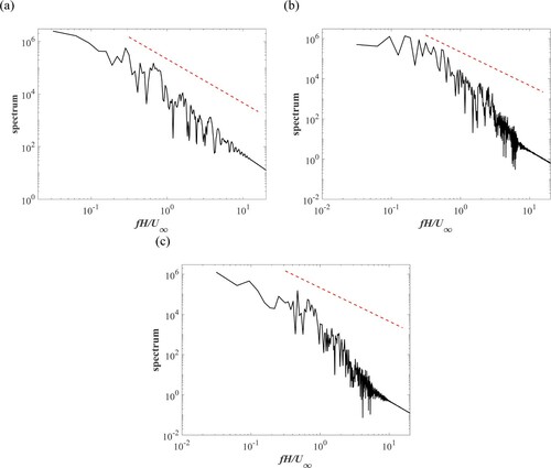
Figure 8. Time histories of $C_D$, $C_L$ for (a) the square rib of Case 3; (c) the trapezoidal rib of Case 9 and (e) the rectangular rib of Case 12 and phase-space plots of $C_D$, $C_L$ for (b) the square rib; (d) the trapezoidal rib and (f) the rectangular rib.

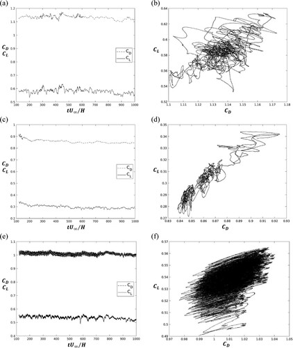
Figure 9. The streamlines of the time- and spanwise-averaged flows for (a) the square rib of Case 3; (b) the trapezoidal rib of Case 9; (c) the rectangular rib of Case 12.

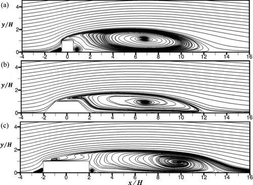
Figure 10. Instantaneous iso-surface of $Q=0.25$ at $t{U}_{\mathrm{\infty }}/H=1000$ for (a) the square rib of Case 3; (b) the trapezoidal rib of Case 9; (c) the rectangular rib of Case 12. (This figure is available in colour online.)

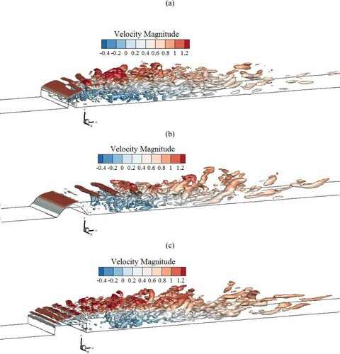
Figure 11. Power spectra density of the cross-stream velocity ($v$) for the square rib at a distance of (a) $L_x/H=0.5$ (b) $L_x/H=3.5$ and (c) $L_x/H=5.5$ to the back face of the rib. (This figure is available in colour online.)

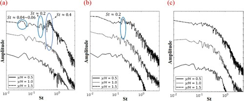
Figure 12. Power spectra density of the cross-stream velocity ($v$) for the trapezoidal rib at a distance of (a) $L_x/H=0.5$ (b) $L_x/H=3.5$ and (c) $L_x/H=5.5$ to the back face of the rib. (This figure is available in colour online.)

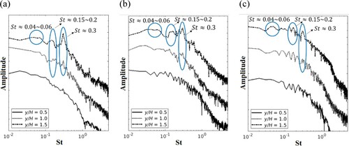
Figure 13. Power spectra density of the cross-stream velocity ($v$) for the rectangular rib at a distance of (a) $L_x/H=0.5$ (b) $L_x/H=3.5$ and (c) $L_x/H=5.5$ to the back face of the rib. (This figure is available in colour online.)

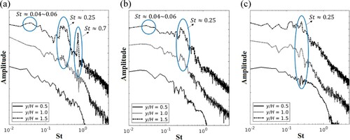
Figure 14. Representation of the snapshots assembling along the (a) streamwise direction and the (b) spanwise direction.

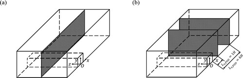
Figure 15. The mean value of ${ϵ}_{ortho}$ of the ten most energetic modes between different sets of snapshots of the velocity modes based on: (a) number of snapshots; (b) $\mathrm{\Delta }{t}_{\mathrm{P}\mathrm{O}\mathrm{D}}$ of the velocity modes.

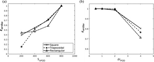
Figure 16. The mean value of ${ϵ}_{ortho}$ of the ten most energetic modes between different sets of snapshots of the pressure modes based on: (a) number of snapshots; (b) $\mathrm{\Delta }{t}_{\mathrm{P}\mathrm{O}\mathrm{D}}$ of the velocity modes.

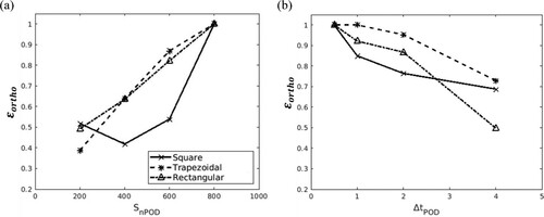
Figure 17. Modal decomposition of the velocities for the square rib: (a) energy of modes; (b) energy contribution of the 20 leading energetic modes; (c) temporal coefficients of Modes 2 and 3 and (d) frequency spectra of Modes 2 and 3; (e) temporal coefficients of Modes 4 and 5 and (f) frequency spectra of Modes 4 and 5.

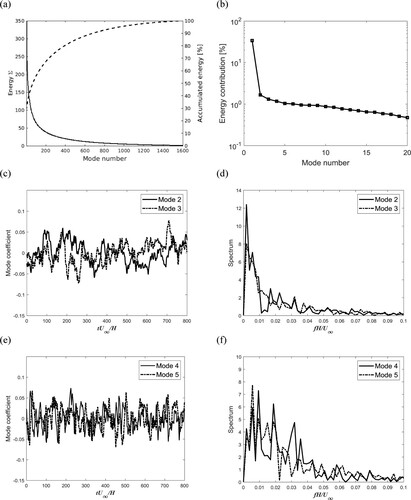
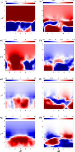
Figure 18. POD modes of the streamwise (a, c, e, g) and cross-stream (b, d, f, h) velocities for the square rib: (a, b) POD Mode 2; (c, d) POD Mode 3; (e, f) POD Mode 4 and (g, h) POD Mode 5. (This figure is available in colour online.)

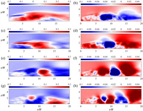
Figure 19. Modal decomposition of the pressure for the square rib: (a) energy of modes, (b) energy contribution of 20 most energetic modes (c) coefficients of Modes 2 and 3 and (d) frequency spectra of Modes 2 and 3.

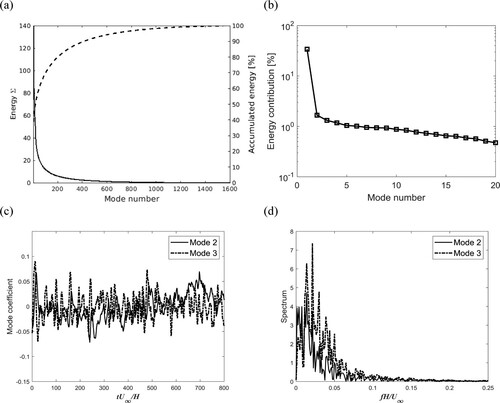
Figure 20. POD modes of the pressure for the square rib: (a) to (h) show POD Modes 2–9. (This figure is available in colour online.)

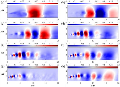
Figure 21. Modal decomposition of the velocities for the trapezoidal rib: (a) energy of modes; (b) energy contribution of most energetic modes; (c) coefficients of Modes 2 and 3 and (d) frequency spectra of Modes 2 and 3; (e) temporal coefficients of Modes 4 and 5 and (f) frequency spectra of Modes 4 and 5.

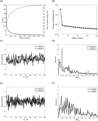
Figure 22. POD modes of the streamwise (a, c, e, g) and cross-stream (b, d, f, h) velocities for the trapezoidal rib: (a, b) POD Mode 2; (c, d) POD Mode 3; (e, f) POD Mode 4 and (g, h) POD Mode 5. (This figure is available in colour online.)

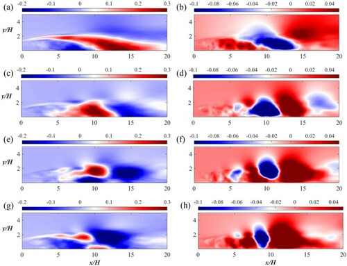
Figure 23. Modal decomposition of the pressure for the trapezoidal rib: (a) energy of modes; (b) energy contribution of the leading energetic modes; (c) coefficients of Mode 2; (d) frequency spectrum of Mode 2; (e) coefficients of Modes 3 and 4; (f) frequency spectra of Modes 3 and 4.

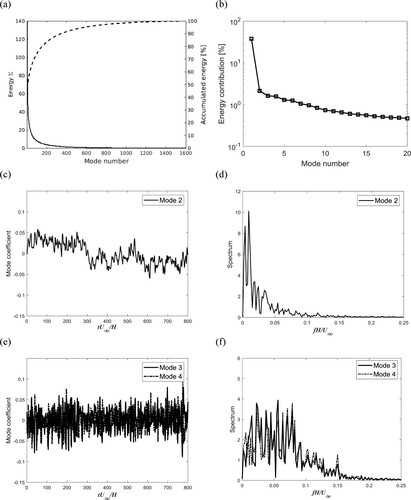
Figure 24. POD modes of the pressure for the trapezoidal rib: (a) to (i) show POD Modes 2–10. (This figure is available in colour online.)

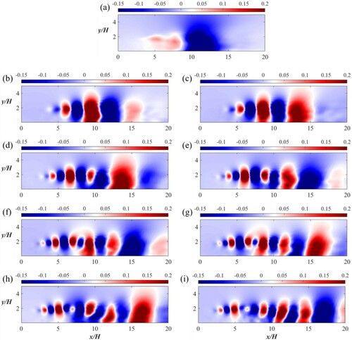
Figure 25. Modal decomposition of the velocities for the rectangular rib: (a) energy of modes; (b) energy contribution of most energetic modes; (c) coefficients of Modes 2 and 3, and (d) frequency spectra of Modes 2 and 3; (e) coefficients of Modes 4 and 5, and (f) frequency spectra of Modes 4 and 5.

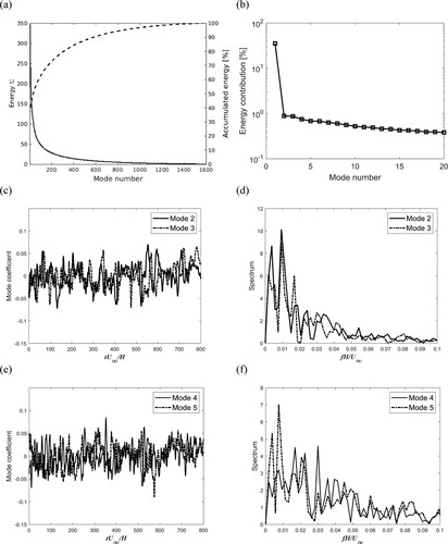
Figure 26. POD modes of the streamwise (a, c, e, g) and cross-stream (b, d, f, h) velocities for the rectangular rib: (a, b) POD Mode 2; (c, d) POD Mode 3; (e, f) POD Mode 4 and (g, h) POD Mode 5. (This figure is available in colour online.)

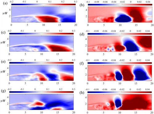
Figure 27. Modal decomposition of the pressure for the rectangular rib: (a) energy of modes; (b) energy contribution of most energetic modes; (c) coefficients of Modes 2 and 3 and (d) frequency spectra of Modes 2 and 3.

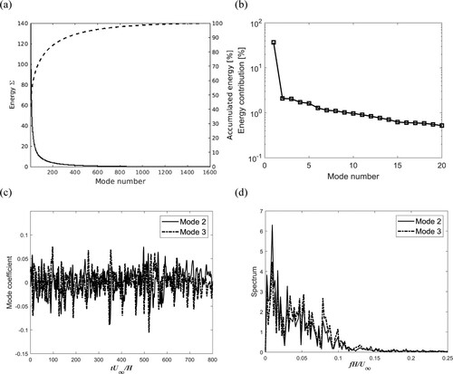
Figure 28. POD modes of the pressure for the rectangular rib: (a) to (h) show POD Modes 2–9. (This figure is available in colour online.)

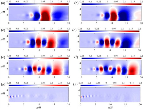
Figure 29. Reynolds stress of four quadrant plots of the POD modes: (a) Mode 2, (b) Mode 3, (c) Mode 4 and (d) Mode 5 for the square rib. (This figure is available in colour online.)

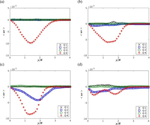
Figure 30. Reynolds stress of four quadrant plots of the POD modes: (a) Mode 2, (b) Mode 3, (c) Mode 4 and (d) Mode 5 for the trapezoidal rib. (This figure is available in colour online.)

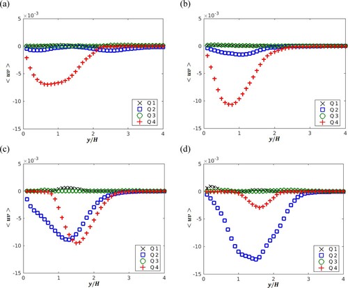
Figure 31. Reynolds stress of four quadrant plots of the POD modes: (a) Mode 2, (b) Mode 3, (c) Mode 4 and (d) Mode 5 for the rectangular rib. (This figure is available in colour online.)

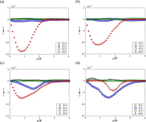
Figure 32. The mean value of ${ϵ}_{ortho}$ of the ten most energetic modes between different sets of snapshots of the velocity modes based on: (a) number of snapshots; (b) $\mathrm{\Delta }{t}_{\mathrm{P}\mathrm{O}\mathrm{D}}$ of the velocity modes at $L_{x,\mathrm{P}\mathrm{O}\mathrm{D}}=1H$ behind the ribs; (c) number of snapshots; (d) $\mathrm{\Delta }{t}_{\mathrm{P}\mathrm{O}\mathrm{D}}$ of the velocity modes at $L_{x,\mathrm{P}\mathrm{O}\mathrm{D}}=6H$ behind the ribs.

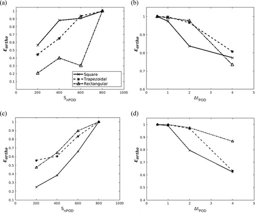
Figure 33. Modal decomposition of the velocities at $L_{x,POD}=1H$: (a) energy of modes; (b) energy contribution of most energetic modes; (c) coefficients of Modes 2 and 3 and (d) frequency spectra of Modes 2 and 3.

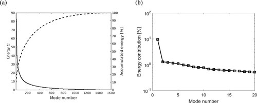
Figure 34. POD modes of the velocities at $L_{x,POD}=1H$ after the square rib: (a, b) POD Mode 2; (c, d) POD Mode 3; (e, f) POD Mode 4; and (g, h) POD Mode 5 with the cross-stream velocities (a, c, e, g) and the spanwise velocities (b, d, f, h). (This figure is available in colour online.)

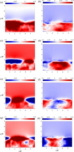
Figure 35. Modal decomposition of the velocities at $L_{x,POD}=6H$: (a) energy of modes, (b) energy contribution of most energetic modes.

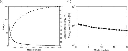
Figure 36. POD modes of the velocities at $L_{x,\mathrm{P}\mathrm{O}\mathrm{D}}=6H$ after the square rib: (a, b) POD Mode 1; (c, d) POD Mode 2; (e, f) POD Mode 3; and (g, h) POD Mode 4 with the cross-stream velocities (a, c, e, g) and the spanwise velocities (b, d, f, h). (This figure is available in colour online.)

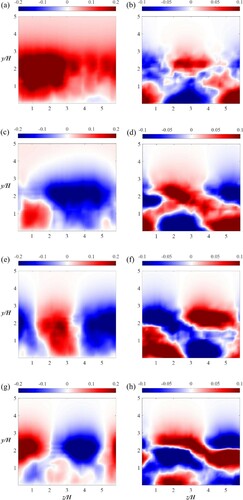
Figure 37. Modal decomposition of the velocities at $L_{x,POD}=1H$ after the trapezoidal rib: (a) energy of modes; (b) energy contribution of most energetic modes.

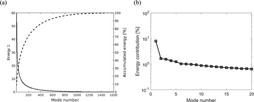
Figure 38. POD modes of the velocities at $L_{x,POD}=1H$ after the trapezoidal rib: (a, b) POD Mode 2; (c, d) POD Mode 3; (e, f) POD Mode 4; and (g, h) POD Mode 5 with the cross-stream velocities (a, c, e, g) and the spanwise velocities (b, d, f, h). (This figure is available in colour online.)

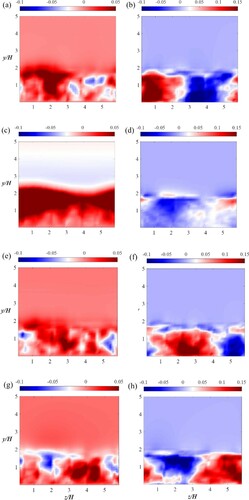
Figure 39. Modal decomposition of the velocities at $L_{x,POD}=6H$ after the trapezoidal rib: (a) energy of modes; (b) energy contribution of most energetic modes.

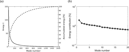
Figure 40. POD modes of the velocities at $L_{x,POD}=6H$ after the trapezoidal rib: (a, b) POD Mode 2; (c, d) POD Mode 3; (e, f) POD Mode 4; and (g, h) POD Mode 5 with the cross-stream velocities (a, c, e, g) and the spanwise velocities (b, d, f, h). (This figure is available in colour online.)

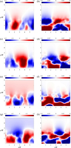
Figure 41. Modal decomposition of the velocities at $L_{x,POD}=1H$ after the rectangular rib: (a) energy of modes; (b) energy contribution of most energetic modes.

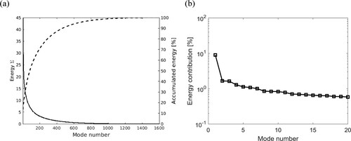
Figure 42. POD modes of the velocities at $L_{x,POD}=1H$ behind the rectangular rib: (a, b) POD Mode 2; (c, d) POD Mode 3; (e, f) POD Mode 4; and (g, h) POD Mode 5 with the cross-stream velocities (a, c, e, g) and the spanwise velocities (b, d, f, h). (This figure is available in colour online.)

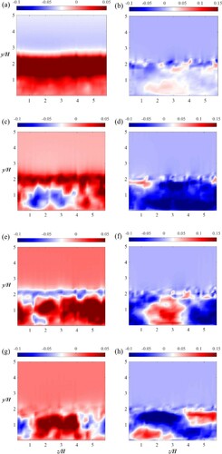
Figure 43. Modal decomposition of the velocities at $L_{x,POD}=6H$ after the rectangular rib: (a) energy of modes, (b) energy contribution of most energetic modes.

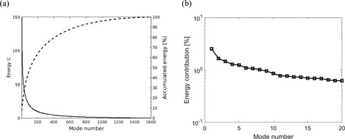
Figure 44. Modal decomposition of the velocities at $L_{x,POD}=6H$ after the rectangular rib: (a, b) POD Mode 2; (c, d) POD Mode 3; (e, f) POD Mode 4; and (g, h) POD Mode 5 with the cross-stream velocities (a, c, e, g) and the spanwise velocities (b, d, f, h). (This figure is available in colour online.)

Liu YZ, Ke F, Sung HJ. 2008. Unsteady separated and reattaching turbulent flow over a two-dimensional square rib. J Fluids Struct. 24(3):366–381.

 Web of Science ®Google Scholar

Tauqeer MA, Li Z, Ong MC. 2017. Numerical simulation of flow around different wall-mounted structures. Ships Offsh Struct. 12(8):1109–1116.

 Web of Science ®Google Scholar