A glacial geomorphological map of the southernmost ice lobes of Patagonia: the Bahía Inútil – San Sebastián, Magellan, Otway, Skyring and Río Gallegos lobes

Figures & data

Figure 1. Location of the study area in southernmost Patagonia (topography shown using shaded SRTM and ETOPO data). Also shown are the present day icefields (numbered) and the Last Glacial Maximum (LGM) limit according to Caldenius (1932); adapted from Singer et al. (2004a).

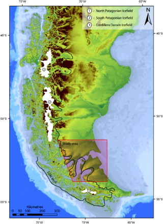
Figure 2. The location and previously hypothesised Marine Isotope Stage (MIS) chronology of drift limits within the study area (Meglioli, 1992; Rabassa et al., 2000; Singer et al., 2004a).

Figure 3. Overview of the study area showing the locations of other figures. Also shown is the area mapped by Lovell et al. (2011), with red boxes highlighting the key areas that have been updated.

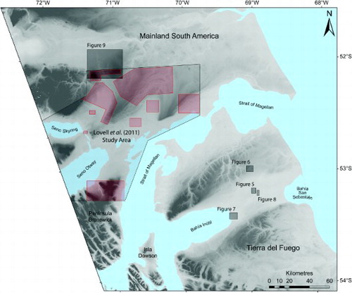
Figure 4. The spatial coverage of different imagery used during mapping. Inset shows the approximate area in which field-checking was conducted. Spatial (pixel) resolution of the different imagery is given in the key.

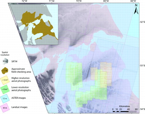
Table 1. Summary of the morphology, appearance and possible errors in mapping geomorphological features.

				Visibility
	Identification criteria			Incr. resolution →
Landform	Morphology	Appearance	Uncertainties	SRTM	Landsat	ASTER	Aerial scans	Aerial photos	Field
Moraine ridges	Distinctive linear or curvilinear ridges deposited at the ice margin or in medial positions.	Arcuate ridges of positive relief (indicated by darker/lighter shading on opposing sides). Often, following the direction of fragmentary ridges leads to the identification of further features.	Medial moraines could have been missed as they would be particularly difficult to identify under these criteria. Ridges and shorelines could potentially be confused. Often only visible in aerial photos.	−	−	−	+	+	+
Subdued moraine topography	Similar to ridges but much wider and with lower elevations, and break-of-slope not as clear.	Subtle changes in topography, with or without change in surface texture, which may be overprinted by more distinct features. Sometimes visible in the field and on SRTM data, very occasionally visible on aerial photographs or Landsat imagery.	Almost certainly missed where ground –truthing was not possible or where they were not visible on SRTM. Difficult to pick-out on the ground and very difficult to identify from imagery.	−	−		−	−	+
Kettle-kame topography	Large belts consisting of disorganised hills and hollows.	Distinctive areas with a pock-marked appearance, consisting of hills and sometimes small lakes. May contain ridges.	Can become discontinuous in lower areas associated with outwash. Sometimes difficult to distinguish drift from terrain that has simply avoided meltwater. Texture can vary significantly (with the presence of kettle lakes, the shape of hills).	−	+	+	+	+	−
Glacial lineations	Linear, parallel landforms aligned to the direction of ice-flow.	Linear features following the inferred direction of ice-flow and generally perpendicular to moraines, often occurring in groups. Not specifically associated with breaks in vegetation and often appear dark on one side and light on the other, indicating positive relief.	Can be short and consequently difficult to identify, even on aerial photos (often invisible on Landsat/ASTER). Fence lines could be mistaken for lineations, and the features are often disrupted by small lakes or (melt)water drainage.		−	−	+	+	−
Irregular hummocky terrain	Areas of small, disorganised hills.	Subtle patches of hills showing no obvious order and only visible in aerial photography.	Only visible on aerial photographs, and therefore could have been missed in areas with no coverage. The boundaries of the hummocky areas can be difficult to discern.				−	+	+
Regular hummocky terrain	Groups of small hills, elongated into small ridges and mirroring patches of small moraine ridges.	Extremely subtle and only visible on high-resolution aerial photography. ‘Order’ is in the apparent form of several hummocks joined into a small ridge. These very short ridges are difficult to discern in the field without the aid of the aerial photography.	Will be missed in areas not covered by high-resolution aerial photography. The organised nature frequently becomes apparent only once numerous ridges have been mapped.					−	+
Irregular dissected ridges	Groups of larger hills or constrained areas of higher relief, sometimes delineated by minor meltwater channels.	Patches of raised topography, often marked by changes in surface texture or vegetation. Sometimes show a mosaic-like pattern, divided by meltwater channels.	Drainage can sometimes give the illusion of ridges. Actual changes in topography are often difficult to see in imagery, so identification can become over-reliant on vegetation changes.		+	+	−	−	−
Eskers	Sinuous ridges, generally running sub-parallel to former ice flow.	Sinuous ridges showing a change in colour due to the shadowing caused by positive relief.	Difficult to identify. Moraine ridges, lineations (especially when deformed) or meltwater channels could be mistaken for eskers.			−	−	−	−
Meltwater channels	Channels formed by large amounts of water from melting ice, often not containing contemporary drainage.	Generally sinuous in form and often occurring in combination with moraine ridges, running against contemporary slope. Frequently do not follow modern drainage routes or contain modern drainage, though this is not universal.	Often filled with contemporary drainage even though fieldwork has demonstrated they are over-sized and were once filled with – or created by – meltwater.	−	−	−	+	+	−
Former shorelines	Raised terraces marking the previous level of a body of water (either sea-level or a lake).	Normally parallel to the coast or an area occupied by a lake and forming concentric lines without relief on one side (shown by shading). Shoreline level is either flat or grades evenly along its length.	Often discontinuous and may become difficult to see when their direction changes, particularly in satellite imagery. May be missed where the location of a palaeo-lake is unknown, and difficult to distinguish from moraine ridges.		−	−	−	−	−
Outwash plains	Large areas of material deposited by meltwater in a flattened, grading plain.	Large, open, approximately flat surfaces, grading to a previous ice limit (marked by moraine ridges, drift, etc), and often dissected by meltwater channels. Generally distinguished by a clear block change in colour and texture on Landsat imagery.	Exact limits of outwash are often difficult to define. Surface grading is often only apparent in the field or over large distances on SRTM. Often form narrow corridors, so can be difficult to distinguish from channels.		+	−	+	+	+
Lakes	Bodies of water surrounded by land (with no link to the sea).	Blue, black or white in colour imagery; white or black in monochrome. Clearly delimited areas often linked to local drainage. Where transient, can show eastward migration patterns linked to westerly winds.	Not always obvious in aerial photos (a counterpart photo is sometimes necessary). Extent of many lakes is very seasonally variable – so their size can vary in different imagery and in the field.		+	+	+	+	+
Volcanic craters	Hollows formed by volcanic eruptions.	Rounded or elliptical and generally creating linear fields.	Unlikely to be mistaken for glacial geomorphology.	−	+	+	+	+	−

The visibility of features on different imagery is also indicated: plus signs mean that features are normally visible; minus signs mean that features may sometimes be visible; and no sign indicates that features are not normally visible on the imagery.

Figure 5. (A) Aerial photograph and (B) the mapped features in the central depression of the BI-SSb lobe. Thin, low moraine ridges (mapped as purple lines) are indicated by the black arrows and drape across the subdued moraine topography (mapped as pink polygons) and lineations (black lines). Locations shown in Figure 3. (C) Field photograph of one of these moraine ridges draped over subdued moraine topography; location shown in (A) and (B) by black circle with arrow. (D) Field photograph of the larger moraines in the Skyring lobe, separated by expansive outwash. Heights in metres above sea level (a.s.l.) are shown for the moraines and outwash plain.

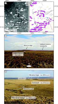
Figure 6. Kettle-kame topography on the northern edge of the BI-SSb lobe. (A) Landsat ETM+ (bands 4, 3, 1) showing the characteristic pock-marked appearance of the drift. (B) Mapped bands of drift (purple polygons), separated by outwash surfaces (yellow polygons). Location shown in Figure 3.

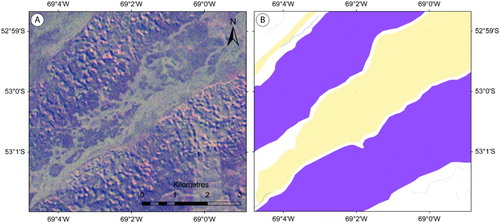
Figure 7. Glacial lineations in the study area. (A) Aerial photograph showing a tightly clustered field of low-relief flutings on the coast of Bahía Inútil and (B) the flutings mapped as black lines. Shorelines are also shown running parallel to the coast (light blue lines). The circle and arrow in (A) show the direction of the field photograph in (C), looking across the flutings which have been highlighted with white lines; locations shown in Figure 3. At the other end of the scale, (D) shows a field photograph of the much larger, sharp-crested drumlins in the Laguna Cabeza del Mar field of the Otway lobe (see map).

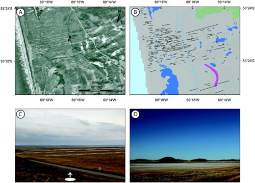
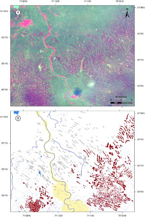
Figure 8. (A) Aerial photograph and (B) mapped equivalent of the regular (yellow lines) and irregular (green polygons) hummocky terrain. Due to their ordered-nature and visibility on higher resolution aerial photographs, the regular hummocky terrain can be mapped as individual line features rather than grouped polygons. Location shown in Figure 3.

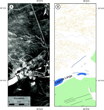
Figure 9. (A) Landsat ETM+ image (bands 4, 3, 1) and (B) mapped equivalent showing the intersection between lineations (black lines) and irregular dissected ridges (brown polygons) between the Skyring (to the south) and Río Gallegos (to the north and west) lobes. Also shown are moraine ridges as purple lines, meltwater channels as blue lines and outwash as yellow polygons. Location shown in Figure 3.

Caldenius, C. C. z. (1932). Las glaciaciones cuaternarias en la patagonia y tierra del fuego. Geografiska Annaler, 14, 1–164. doi: 10.2307/519583

 Google Scholar

Singer, B. S., Ackert, R. P., & Guillou, H. (2004a). 40ar/39ar and k-Ar chronology of pleistocene glaciations in patagonia. Geological Society of America Bulletin, 116, 434–450. doi: 10.1130/B25177.1

 Web of Science ®Google Scholar

Meglioli, A. (1992). Glacial geology and chronology of southernmost patagonia and tierra del fuego, argentina and chile, Geology. Lehigh.

 Google Scholar

Rabassa, J., Coronato, A., Bujalesky, G., Salemme, M., Roig, C., Meglioli, A., Heusser, C., Gordillo, S., Roig, F., Borromei, A., & Quattrocchio, M. (2000). Quaternary of tierra del fuego, southernmost south america: An updated review. Quaternary International, 68–71, 217–240. doi: 10.1016/S1040-6182(00)00046-X

 Web of Science ®Google Scholar

Lovell, H., Stokes, C. R., & Bentley, M. J. (2011). A glacial geomorphological map of the seno skyring-seno otway-strait of magellan region, southernmost patagonia. Journal of Maps, 7, 318–339. doi: 10.4113/jom.2011.1156

 Web of Science ®Google Scholar