Figures & data
Figure 1. Location of the study area.
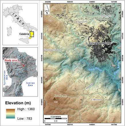
Figure 2. Reference descriptions for the weathering classes (modified from CitationBorrelli et al., in press).
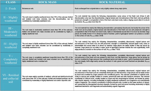
Figure 3. Data collection from observations and measurements at the checkpoints for each cut slope surveyed (modified from CitationGullà & Matano, 1997).
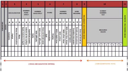
Figure 4. Morphological units (a) and slope map (b) of the study area.
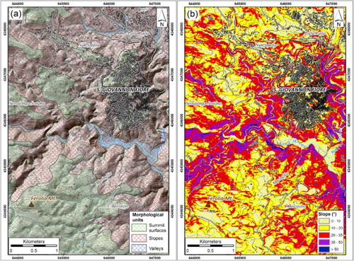
Figure 5. Geo-structural map of the study area: (a) panoramic view of the San Giovanni in Fiore town; (b) Upper Pliocene–Middle Pleistocene clastic deposits; (c) granitoid rocks (Palaeozoic). Notes: (1) alluvial deposits; (2) Upper Pliocene–Middle Pleistocene alternating sands and conglomerates; (3) granitoid rocks with mainly granitoid composition (Palaeozoic); (4) normal fault; (5) left-lateral transcurrent fault reactivated as normal fault; (6) fault with undetermined kinematics; (7) low-angle thrust.
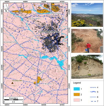
Figure 6. Examples of faults surveyed in the study area at the macro- and meso-scale: (a) panoramic view of the right slope of the Arvo river and some faults related to the main fault systems; (b) N–S transpressive faults; (c) N–S right-lateral transpressive faults; (d) last kinematics on the N–S fault plane in the Pleistocene conglomerates; (e) left-lateral striae on the NW–SE fault plane; (f) ancient overthrust; (g) NW–SE fault zone with associated thick fault gouge.
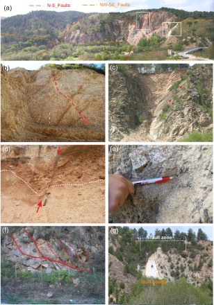
Figure 7. Weathering grade and geotectonic map of the study area. Notes: (1) alluvial deposits; (2) conglomerates and relative covers; (3) class VI; (4); class V; (5) class IV; (6) class III; (7) normal fault; (8) left-lateral transcurrent fault reactivated as normal fault; (9) fault with undetermined kinematics; (10) uncertain thrust; (11) studied weathering profiles; (12) samples collected for the petrographic analyses.
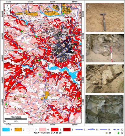
Figure 8. Schematic weathering profile reconstructed by the cut slopes survey: (a and b) corestones outcropping on the ground surface near Mt. Ferolia and near Marinella area, above 1100 m a.s.l.; (c) examples of aplitic dike of class III immersed in class V, generally widespread above 1000 m a.s.l.; (d) typical features of the cut slopes observed between 1360 and 1050 m a.s.l; (e–g) typical features of the cut slopes observed (e) from 1050 to 1000 m a.s.l, (f) from 1000 to 930 m a.s.l, (g) from 930 to 783 m a.s.l.
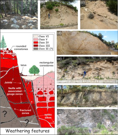
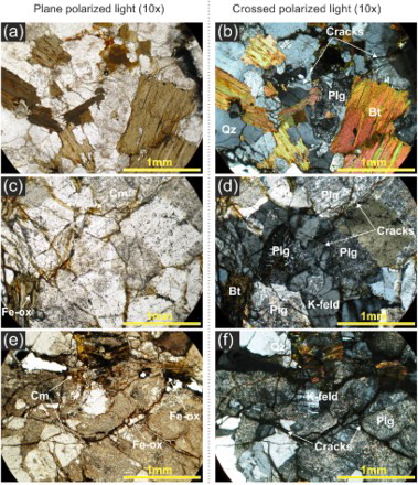
Figure 9. Photomicrographs of weathering stages for the studied granitoid: (a and b) moderately weathered sample (class III); (c and d) highly weathered sample (class IV); (e and f) completely weathered sample (class V). K-feld, K-feldspar; Plg, plagioclase; Chl, chlorite; Bt, biotite; Qtz, quartz; Cm, clay minerals; Fe ox, Fe oxides.