Figures & data
Figure 1. Location map of the studied area in central Patagonia. Boxes indicate the location and number of additional figures. Inset shows the extent of the Patagonian Ice Sheet (PIS) at the Last Glacial Maximum (LGM); redrawn after CitationSinger et al. (2004). The −125 m contour provides an indication of the approximate sea level drop at the LGM (e.g. CitationLambeck, Rouby, Purcell, Sun, & Sambridge, 2014; CitationPeltier & Fairbanks, 2006; CitationYokoyama, De Deckker, Lambeck, Johnston, & Fifield, 2001). NPI: North Patagonian Icefield; SPI: South Patagonian Icefield; CDI: Cordillera Darwin Icefield. Contemporary icefield limits extracted from the ‘Randolph Glacier Inventory’ dataset (CitationPfeffer et al., 2014).
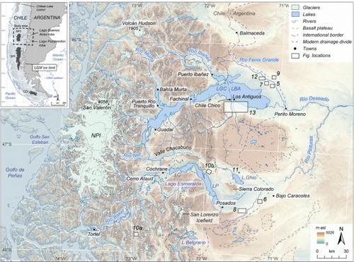
Figure 2. Extent and resolution of previous glacial geomorphological mapping studies, with mapped features listed in .
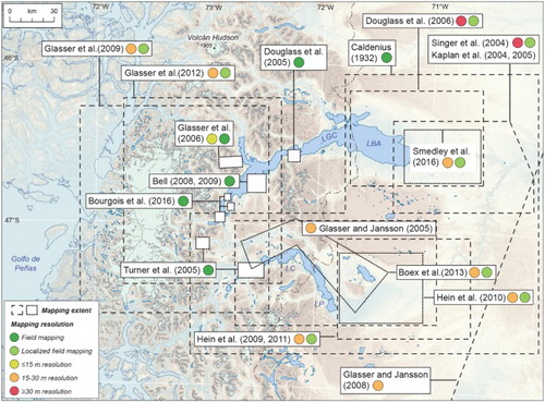
Table 1. Features mapped in previous studies.
Table 2. Summary of glacial geomorphology mapped in this study and criteria used in landform identification.
Table 3. Landforms mapped in this study classified according to depositional environment.
Figure 3. Major glacier limits and compilation of associated dating evidence based on previous studies. Cosmogenic nuclide exposure ages are presented as reported in original publications; however, where available, we report recalculated ages obtained from the use of southern hemisphere production rates (e.g. CitationKaplan et al., 2011; CitationPutnam et al., 2010). Luminescence ages are presented as reported in original publications. Published 14C determinations were recalibrated in Oxcal v4.3 (CitationBronk Ramsey, 2009) using the southern hemisphere calibration curve of CitationHogg et al. (2013). Arrows represent major ice lobe flow lines (CitationGlasser & Jansson, 2005).
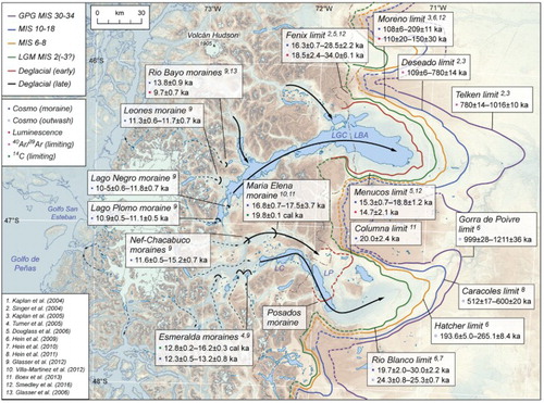
Figure 4. Mapping legend to accompany . Note that on some figures, certain layers (e.g. ‘morainic complexes or deposits’) are not shown to enhance the visual clarity of our landform interpretations. Contemporary glacier extents were extracted from the ‘Randolph Glacier Inventory’ dataset presented in CitationPfeffer et al. (2014).
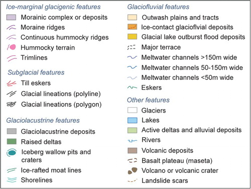
Figure 5. (A) Satellite image (DigitalGlobe 2015; ESRI™) and (B) mapped moraine ridges and outwash deposits from the northern margin of the LGC-BA lobe. Outwash occurs within narrow meltwater channels incised through moraines (left of image) or as broader lateral corridors between moraine sequences (centre left of image). Moraines are locally dissected by former meltwater streams (right of image) which feed into broad sandur plains. (C) View across latero-frontal moraine arc east of Puerto Ibañez with higher elevation (older) moraine sequence in distance (right of image).
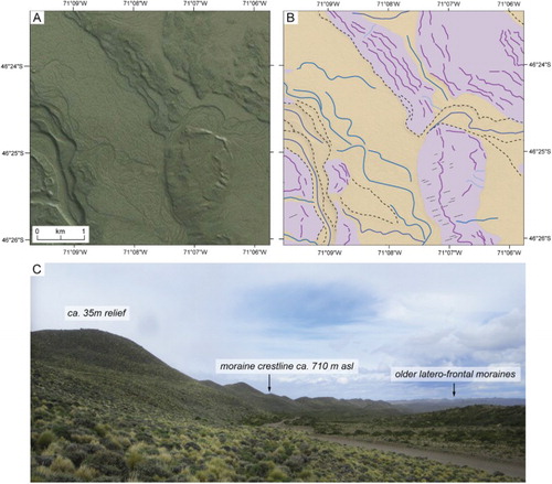
Figure 6. (A) Satellite image (DigitalGlobe 2015; ESRI™) and (B) continuous hummocky ridges mapped along the southern LC-P ice lobe margin. The image shows numerous short ridges and hummocks that connect to generate longer ice-margin parallel chains when viewed in planform. Sequences of closely spaced ridges are separated by narrow lateral outwash corridors, whilst individual ridges may be separated by minor marginal meltwater channels of <50 m wide. The outer ridges (bottom right of image) are heavily dissected by meltwater channels which feed a lateral sandur plain. (C) View across continuous hummocky ridge chain, showing variable hummock height and lengths, and proglacial outwash deposits.
Figure 7. (A) Satellite image (DigitalGlobe 2013; ESRI™) and (B) mapped hummocky terrain on the northern LGC-BA ice lobe margin. These small-scale hummocks are largely chaotic but may be organized into crude arcuate bands (top left of image) that are interspersed with low-relief push moraine ridges.
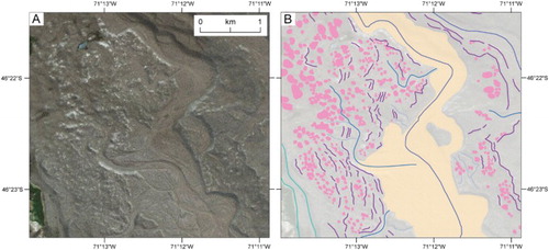
Figure 8. (A) Context for landform interpretation along the southern LC-P ice lobe margin, east of Posados. Late LGM glacier and proglacial lake limit after CitationHein et al. (2010), based on the identification of lacustrine deposits (black circles). At the time of the reconstruction, CitationHein et al. (2010) suggest ice was grounded around a prominent north–south trending bedrock step, and experienced insufficient flux to fully occupy the upper basin. The lake level contour (625 m a.s.l) was extracted from an ASTER-GDEM model. The extent of (B) and (C) is indicated by the dashed white box. (B) Satellite image (DigitalGlobe 2013; ESRI™) and (C) mapped landforms, showing a complex arrangement of geomorphic features. The right-hand section of the image shows an assemblage of densely spaced circular or oval-shaped mounds and linear ridges that display morphological resemblance with examples of ice-stagnation hummocky terrain (CitationEyles et al., 1999; CitationBoone and Eyles, 2001). The hummock assemblage merges into a large complex of inferred iceberg wallow pits and craters, which exhibit deep semi-circular to elongate depressions and are enclosed by high-relief rim ridges or lateral berm ridges (e.g. CitationBarrie et al., 1986; CitationWoodward-Lynas et al., 1991). Low-relief hummock chains are interpreted as moat line ridges deposited at the margins of a small ice-contact lake ice (cf. CitationHall, Hendy, & Denton, 2006). Inferred moat line ridges occur outside the limits of hummocky terrain, and along the ice-contact face of prominent sharp-crested ridges. Their distribution and ‘shoreline-like’ pattern (A) is consistent with the perimeter and estimated water level of the proglacial lake system mapped by CitationHein et al. (2010).
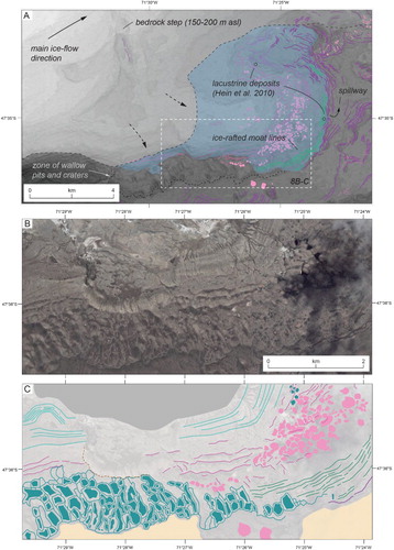
Figure 9. (A) Satellite image (DigitalGlobe 2012; ESRI™) and (B) mapped landforms on the northern margin of the LGC-BA lobe. Image shows saw-tooth push moraines and straight-to-sinuous inset ridges that align sub-parallel to former ice-flow direction, and are interpreted as preserved till eskers as recorded on some modern glacier forelands (CitationChristoffersen et al., 2005; CitationEvans et al., 2016).
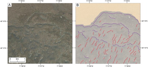
Figure 10. Examples of glacial lineations from across the study area. (A) Satellite image (DigitalGlobe 2014; ESRI™) and (B) mapped lineations formed in bedrock south of Los Ñadis. (C) Satellite image (DigitalGlobe 2015; ESRI™) and (D) mapped lineations formed in sediment at the junction of Valle Chacabuco and the Pueyrredón basin.
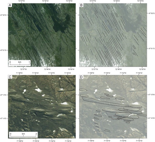
Figure 11. (A) Satellite image (DigitalGlobe 2017; Bing Maps™) from the northern margin of the LC-P lobe and (B) mapped landforms. The image shows a prominent, positive relief, sinuous ridge interpreted as an esker, alongside multiple smaller esker ridges. Ice-flow direction was from left to right.
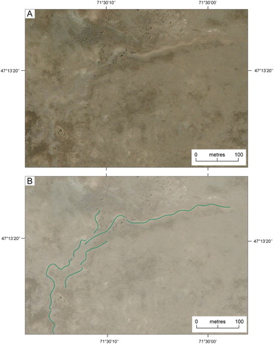
Figure 12. (A) Satellite image (DigitalGlobe 2013; ESRI™) from the northern margin of the LGC-BA lobe and (B) interpretation of the glacial geomorphology. The image shows push moraine ridges, inset eskers and sediment flutings. The inferred eskers range from sinuous ridges that are either isolated or occur within complex networks (lower right of image), to more enigmatic, near-straight ridges and conical mounds (centre of image) of comparatively high relief (C).
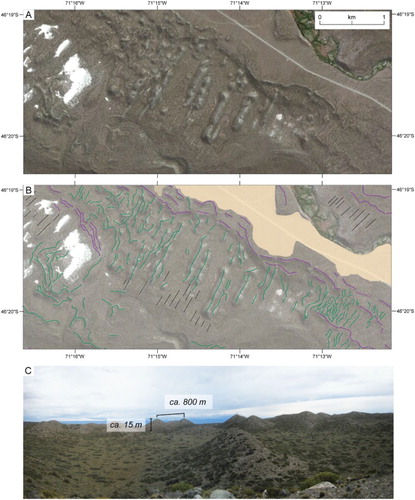
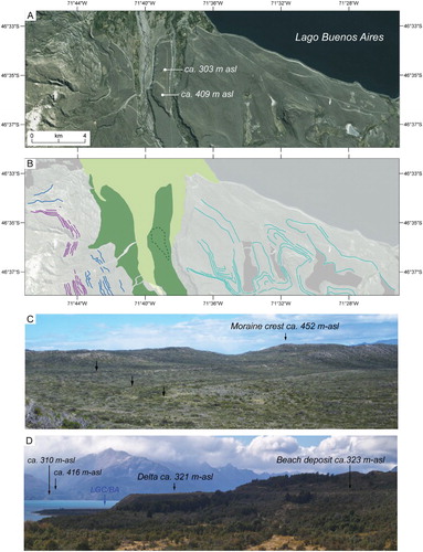
Figure 13. (A) Satellite image (DigitalGlobe 2014; ESRI™) and (B) mapped glaciolacustrine landforms along the southern margin of Lago General Carrera–Buenos Aires. Features include raised deltas, wave-cut lake shorelines and areas of lacustrine sediment accumulation within palaeolake embayments. Also note the high-level lateral moraine ridges and marginal meltwater channels of the southern LGC-BA lobe margin. Field photos of (C) former lake shorelines cut into glacigenic deposits and (D) raised lacustrine deltas and adjacent beach deposits formed in the mouths of tributary valleys of Lago General Carrera–Buenos Aires. The ca. 310 and 321 m deltas are coeval though have experienced different amounts of postglacial uplift. The ca. 416 m delta pre-dates the lower elevation features and records stepped lake level lowering.