Figures & data
Figure 1. Ganymede Voyager and Galileo Global Mosaic, Mercator projection. The dashed yellow lines define the boundaries of the leading (LH in figure) and the trailing (TH) hemispheres at the W and E, respectively.
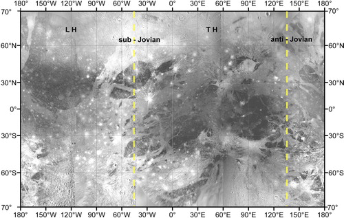
Figure 2. Grooved terrain. The red arrows show groove examples.
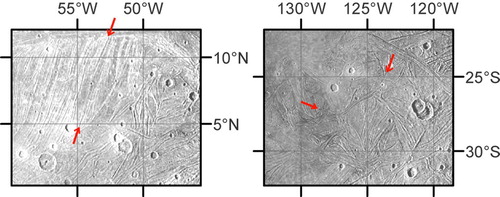
Figure 3. Grooves global mapping, Mercator projection. A total of 14,707 identified regional grooves is shown.
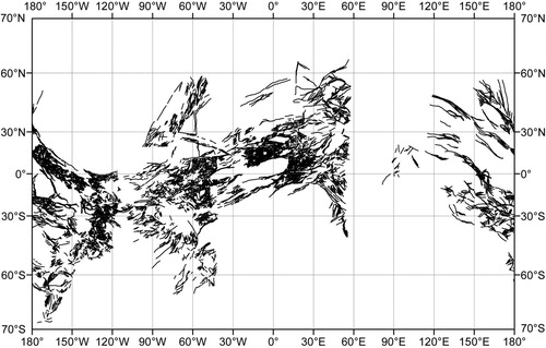
Figure 4. Cumulative azimuthal analysis of the mapped grooves. The Gaussian Parameter are reported in the lower left table: the number of Gaussian peaks (#), the percentage of occurrence (%), the Normalized Height (NorH), the Maximum height (MaxH), the azimuth, and the standard deviation (sd). The preferential Gaussian peaks represent the azimuthal interval for the classification into super-systems.
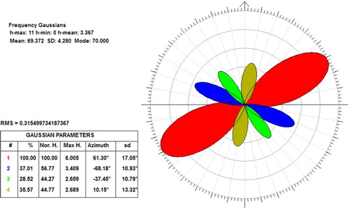
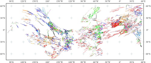
Figure 5. Azimuthal grid analysis, Equidistant Cylindrical projection. Circles of the grid are represented as their mean dimension at the equator. In the circle centres are shown the classified Gaussians; in background the mapped grooves are represented. The legend explains the mean azimuth and the peak number (n) of each system of the grid analysis.
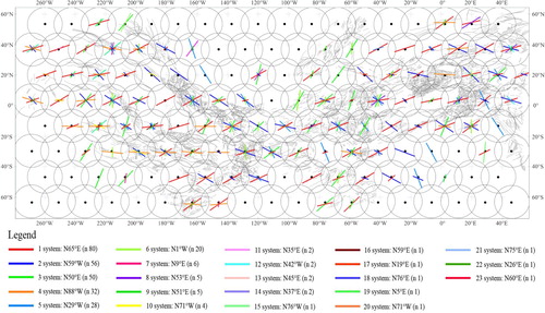
Figure 6. Identification of the 23 main systems associated to super-systems shown in . Colour-coded legend is reported in ; black lines represent unclassified groove elements.