Harmonizing multi-source backscatter data using bulk shift approaches to generate regional seabed maps: Bay of Fundy, Canada

Figures & data

Figure 1. MBES data coverage for individual surveys in the Bay of Fundy, Canada. Each colour group represents surveys collected by the same vessel, with different shades representing various years. Note that CSL Plover/CSL Heron data were obtained as a combined pre-processed grid. A more comprehensive list of individual backscatter mosaic coverages and their respective survey year is provided in the Main Map.

A regional map of the Bay of Fundy, Canada, overlain by multibeam echosounder survey coverages. There are 15 individual backscatter mosaics. Mosaics collected by the same survey vessel share the same colour but have different shades representing varying survey years.

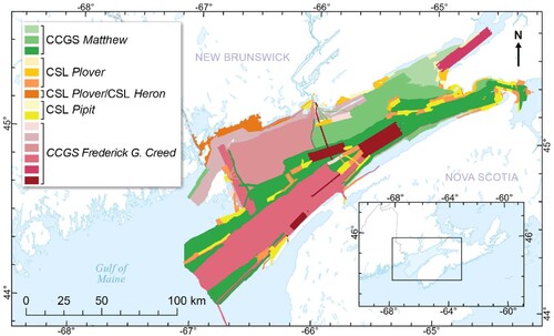
Table 1. Summary of surveys and multibeam echosounders used to collect data that were reprocessed and used in this study (Hughes Clarke et al., 2008; Parrot et al., 2010a, 2010b, 2010c, 2010d, 2010e; Parrott et al., 2013; Todd et al., 2011b).

Vessel	Survey years	Sonar model	Operating frequency (kHz)
CCGS Frederick G. Creed	1996, 1999	EM1000	95
CCGS Frederick G. Creed	2006, 2007, 2008	EM1002	93/98
CCGS Matthew	2007, 2008, 2009	EM710	71-97
CSL Heron	2006, 2007	EM3002	300
CSL Plover	2007, 2008, 2009	EM3002	300
CSL Pipit	2007, 2008	EM3002	300

Figure 2. Summary of the multi-step bulk shift process used to create the final harmonized backscatter map for the Bay of Fundy. More comprehensive details on the harmonization order and model information for each bulk shift used to produce the harmonized backscatter mosaic can be found in the Supplementary Material S2.

A flow diagram summarizing the order in which individual mosaics were harmonized to create the final backscatter mosaic. The more extensive mosaics which were collected using the same survey vessel were harmonized first, followed by less extensive and isolated mosaics.

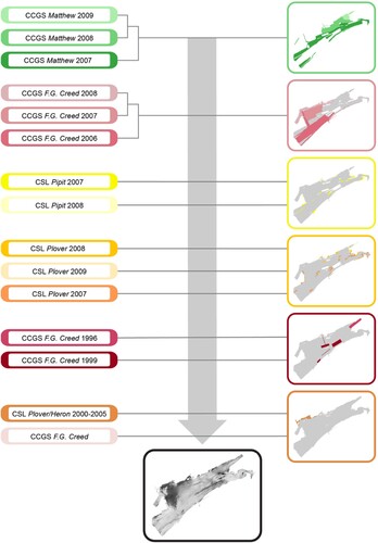
Figure 3. Line artefacts present in the CCGS Frederick G. Creed (a) were corrected using a modified bulk shift approach to produce a corrected mosaic (b).

A side-by-side comparison of backscatter mosaics before and after correcting line artefacts present within the datasets. Figure A on the left showcases three line artefacts present within various datasets where the raster cells have backscatter values that are higher than the surrounding cells. The right image, representing the post-harmonization results, has no obvious remnants of the line artefacts and the larger mosaic remained unaffected.

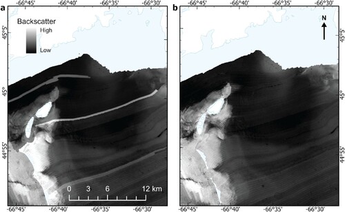
Figure 4. An intercept-only (i.e. ‘mean’) error model was used for harmonizing all same-system corrections such as the 2008 and 2009 CCGS Matthew data shown here. Backscatter measurements for two datasets are extracted at areas where raster cells overlap (a). Then, the mean backscatter error is calculated between datasets and is used to apply bulk corrections to the ‘shift’ dataset to produce a continuous mosaic (b).

A side-by-side comparison of backscatter mosaics before and after applying a bulk shift correction using an intercept-only error model. The bulk shift harmonization method uses the area of overlap between two layers for relative statistical calibration. Image A on the left highlights this area of overlap in red. Image B on the right shows the post-harmonization results, and visually appears to be a continuous backscatter layer with no obvious divisions between the two original layers.

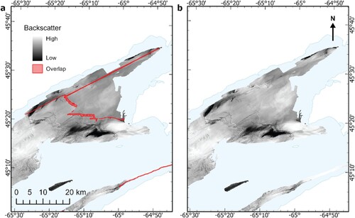
Figure 5. Linear relationship between depth and backscatter error ($\mathrm{slope}=0.02$dB/m) for the Pipit 2007 data, compared to the combined CCGS Frederick G. Creed/Matthew data.

A scatterplot depicting a positive linear relationship between depth and backscatter error values for two datasets.

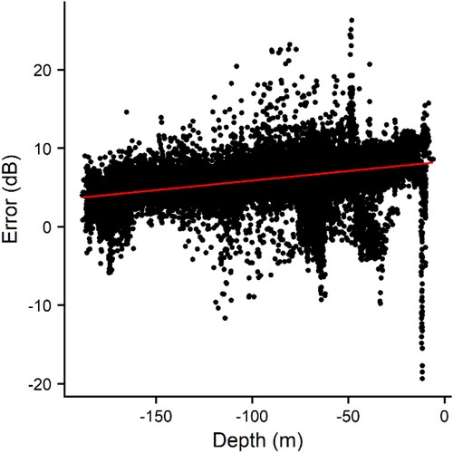
Figure 6. Data from a previous harmonized mosaic (a; Hughes Clarke et al., 2008) were incorporated where legacy data were unavailable. The linear bulk shift error model (b) rescales the data to match the ‘target’, even using values on arbitrary non-dB scales (e.g. 0-255). The regression line indicates the modelled error where the datasets overlap, which also varies as a function of water depth (indicated by the error band). Following correction, the datasets are mosaicked (c), and data distributions are compared between datasets at the area of overlap (d).

Read the detailed description of this figure

Four images including two maps showing two datasets before and after harmonization, along with a scatterplot of the results of the bulk shift error model and a box plot of the data distributions compared between the two. Fig. 6 Long Description: Figure A in the top left (a) is a map showing an example of where data from a previous harmonized mosaic was incorporated where legacy data were unavailable to expand the coverage of the map. Figure B in the top right is a scatter plot which shows the results of the linear bulk shift error model applied to the data and highlights a negative linear relationship. A regression line is plotted with an error band, which indicates the modelled error where the datasets overlap, which also varies as a function of water depth. Figure C in the bottom left is a map of the same two datasets from Figure A after they have been harmonized. Figure B in the bottom right is a boxplot showing the data distributions compared between datasets at the area of overlap.

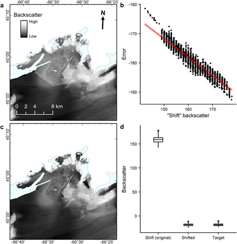
Figure 7. ‘Mixed sediment’ backscatter value distributions for each MBES dataset (a) before and (b) after bulk shift harmonization.

Two boxplots showing the backscatter value distributions for each MBES dataset before and after bulk shift harmonization. The boxplot on the left shows the before results, and the plot on the right shows the after results.

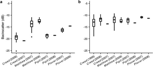
Table 2. Results of one-way randomization ANOVA tests for differences in backscatter between datasets for each seabed class.

Class	Original			Harmonized
	$n$	$F$	$p$	$n$	$F$	$p$
Sand	47	0.9716	0.4748	68	1.7560	0.1049
Gravelly sand	20	3.1466	0.0431*	22	0.7713	0.4845
Mixed sediments	73	34.5805	0*	77	0.9325	0.4344
Tidal scoured mixed sediments	12	3.5411	0.0699	12	0.8949	0.5100
Silty gravel with anemones	15	6.6052	0.0041*	15	1.6008	0.2614
Silt	7	2.0141	0.4012	7	0.2053	0.7372
Bedrock and boulders^†	–	–	–	–	–	–

*Significant at $\alpha =0.05$_.

^† Not enough samples for randomization tests.

Hughes Clarke, J. E., Iwanowska, K. K., Parrott, R., Duffy, G., Lamplugh, M., & Griffin, J. (2008). Inter-calibrating multi-source, multi-platform backscatter data sets to assist in compiling regional sediment type maps: Bay of Fundy. In Proceedings of the Canadian Hydrographic Conference and National Surveyors Conference 2008 (p. 22). Victoria, BC, Canada.

 Google Scholar

Parrot, D. R., Beaver, D., Fraser, P., Hayward, S., Patton, E., Griffin, J., & Lamplugh, M. (2010a). Cruise Report Matthew 2008030 and 2008042 Bay of Fundy 17 September to 3 November 2008 (Open File No. 6229). Geological Survey of Canada.

 Google Scholar

Parrott, D. R., Beaver, D., Hayward, S., & Patton, E. (2010b). Cruise Report Creed 2008030 - Bay of Fundy 22 June −26 July 2008 (Open File No. 6227). Geological Survey of Canada.

 Google Scholar

Parrott, D. R., Duffy, G., Girouard, P., Hayward, S., Patton, E., MacGowan, G., Rodger, G., Sabadash, K., & Smith, A. (2010c). Cruise Report Creed IML 2006-030 - Bay of Fundy 12 June - 17 August 2006 (Open File No. 5584). Geological Survey of Canada.

 Google Scholar

Parrot, D. R., Fraser, P., Hayward, S., Patton, E., & Griffin, J. (2010d). Cruise Report Matthew 2009053 Bay of Fundy 9 October to 4 November 2009 (Open File No. 6473). Geological Survey of Canada.

 Google Scholar

Parrot, D. R., Patton, E., Hayward, S., Duffy, G., MacGowan, B., & Rodger, G. (2010e). Cruise Report Creed IML 2007-022 and IML 2007-023 Bay of Fundy 12 July - 30 August 2007 (Open File No. 6475). Geological Survey of Canada.

 Google Scholar

Parrott, D. R., Hayward, S., Fraser, P., Lamplugh, M., & Griffin, J. (2013). Cruise Report Matthew 2007006 and 2007016: Bay of Fundy 3 May - 16 June 2007 (Open File No. 6474). Geological Survey of Canada. https://doi.org/10.4095/292368

 Google Scholar

Todd, B. J., Shaw, J., Parrott, D. R., Hughes Clarke, J. E., Cartwright, D., & Hayward, S. E. (2011b). Backscatter strength and shaded seafloor relief, Bay of Fundy, sheet 1, offshore Nova Scotia - New Brunswick (Open File No. 7024). Geological Survey of Canada. https://doi.org/10.4095/289508

 Google Scholar

Data availability

The authors confirm that all data supporting the results and analyses presented within the article are available upon reasonable request.