Red sea urchins (Echinus esculentus) and water flow influence epiphytic macroalgae density

Figures & data

Figure 1. Map showing the 636 stations with kelp (Laminaria hyperborea) recorded in northern Norway (Nordland County), from Salten in the south (southernmost station at 66.8°N) to the Lofoten area in the north (northernmost station at 68.6°N).

Table I. Mean, standard deviation (SD), minimum and maximum values for the environmental variables used as predictors in the analyses.

Predictors	Mean	SD	Minimum	Maximum
Depth (m)	11.8	7.3	−0.03	37.6
Terrain curvature, 250 m calculation window (m)	3.5	6.9	−25.8	25.3
Terrain curvature, 500 m calculation window (m)	9.5	13.1	−53.6	54.5
Terrain curvature, 1 km calculation window (m)	17.8	21.9	−96.3	94.9
Wave exposure index	371,495	248,007	2488	1,020,289
Mean current speed (m/s)	0.03	0.03	0.00	0.33
Maximum current speed (m/s)	0.28	0.14	0.10	1.50
Mean temperature (°C)	3.38	0.41	2.28	4.88
Maximum temperature (°C)	5.16	0.59	3.93	6.96
Mean salinity (psu)	34.02	0.15	33.51	34.41
Maximum salinity (psu)	34.26	0.14	33.80	34.57

Table II. Correlation matrix (Pearson's R) for the environmental variables.

	Max. temp	Mean temp	Max. sal	Mean sal	Depth	Latitude	Slope	Curv (250 m)	Curv (500 m)	Curv (1 km)	Wave	Max. curr
Mean temp	0.488
Max. sal	−0.485	0.240
Mean sal	−0.587	0.098	0.897
Depth	−0.073	0.041	0.168	0.199
Latitude	0.364	0.489	0.181	0.161	0.187
Slope	−0.177	−0.081	0.212	0.214	0.089	−0.044
Curv (250 m)	−0.290	−0.041	0.164	0.207	−0.315	−0.102	0.139
Curv (500 m)	−0.452	−0.114	0.248	0.300	−0.253	−0.161	0.187	0.911
Curv (1 km)	−0.579	−0.144	0.353	0.401	−0.178	−0.169	0.155	0.719	0.896
Wave	−0.275	−0.224	0.061	0.200	0.261	−0.305	0.032	−0.038	0.039	0.042
Max. curr	0.025	0.045	0.052	0.018	0.165	−0.015	−0.082	0.066	0.064	0.038	0.182
Mean curr	0.010	−0.056	−0.051	−0.060	0.104	−0.044	−0.127	0.071	0.027	−0.009	0.171	0.663

Temp, temperature; sal, salinity; curv, terrain curvature with 200, 500 and 1 km calculation windows; wave, wave exposure index; curr, current speed.

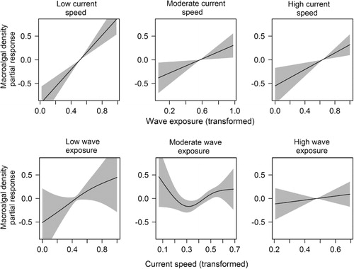
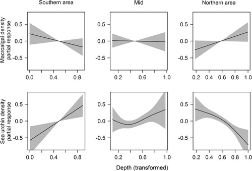
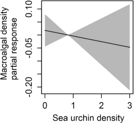
Table III. Overview of the best models explaining the density of the epiphytic macroalgae on kelp (Laminaria hyperborea) stipes and the density of red sea urchins (Echinus esculentus). We present the models with ΔAICc < 4, i.e. the models receiving equally good support from the data (according to Burnham et al. 2011).

Model		AICc	ΔAICc
Density of epiphytic macroalgae
1	wave + sal + depth × wave + curr + depth × lat + urchin + wave × curr + curv + lat + depth + temp	1091.1	0
2	wave + sal + depth × wave + curr + depth × lat + urchin + wave × curr + curv + lat + depth	1091.2	0.1
3	wave + sal + depth × wave + curr + depth × lat + urchin + wave × curr + lat + depth	1095.1	3.9
Density of sea urchins
1	depth × lat + depth + lat + curv(1km)	1337.4	0
2	depth × lat + depth + lat	1337.4	0.34

Wave, wave exposure index; sal, mean salinity; curr, maximum current speed; lat, latitude; urchin, red sea urchin (Echinus esculentus) density; curv, terrain curvature with 250 m calculation window; temp, mean temperature; curv(1km), terrain curvature with 1 km calculation window, × indicates interactions

Figure 2. Partial response curves (with 95% confidence interval) showing the density of epiphytic macroalgae on kelp (Laminaria hyperborea) stipes against wave exposure at low, moderate and high maximum current speed levels (upper panel) and against maximum current speed at low, moderate and high wave exposure index levels (lower panel). Predictor variables were transformed to zero skewness at a 0–1 scale in order to achieve normally distributed residuals.

Figure 3. Partial response curves (with 95% confidence interval) showing the density of epiphytic macroalgae on kelp (Laminaria hyperborea) stipes (upper panel) and the density of red sea urchins (Echinus esculentus, lower panel), both plotted against depth in the southern, mid and northern regions of the study area. Predictor variables were transformed to zero skewness at a 0–1 scale in order to achieve normally distributed residuals.

Figure 4. Partial response curves (with 95% confidence interval) showing the density of epiphytic macroalgae on kelp (Laminaria hyperborea) stipes against the density of red sea urchins (Echinus esculentus). Density classes are 0: absent, 1: single individuals, 2: scarce (∼2–3 ind.) and 3: common/moderately dense (∼4–6 ind.).

Burnham KP, Anderson DR, Huyvaert K. 2011. AIC model selection and multimodel inference in behavorial ecology: Some background observations and comparisons. Behavioral Ecology and Sociobiology 65:23–35.10.1007/s00265-010-1029-6

 Web of Science ®Google Scholar