708
Views
5
CrossRef citations to date
0
Altmetric
Original Articles

Composition and vertical distribution of the motile epifauna on a vertical rock wall in Gullmarsfjorden, western Sweden, using an alternative sampling approach

&
Pages 107-117 | Accepted 03 Jan 2005, Published online: 18 Feb 2007

Figures & data

Figure 1. Location of the sampling site in Gullmarsfjorden on the Swedish west coast. The dotted line represents the 100 m isobath. KMRS=Kristineberg Marine Research Station.
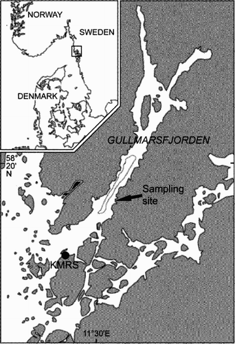
Figure 1. Location of the sampling site in Gullmarsfjorden on the Swedish west coast. The dotted line represents the 100 m isobath. KMRS=Kristineberg Marine Research Station.

Table I. Efficiency of the suction sampler. The number of taxa after an ordinary sampling and after an additional 3 min sampling at the same spot.

Table II. Taxa found on the three sampling occasions.

Figure 2. Mean abundance of taxonomic groups, expressed as individuals per 0.1 m2. The error bars represent+standard error values.
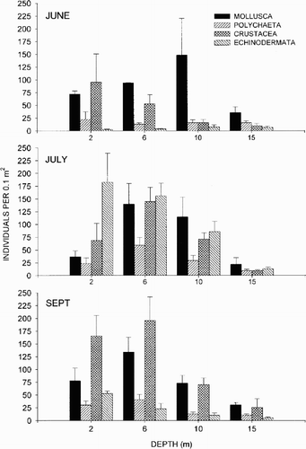
Figure 2. Mean abundance of taxonomic groups, expressed as individuals per 0.1 m2. The error bars represent+standard error values.

Figure 3. a) Diversity (Shannon-Wiener index), b) evenness expressed by Hill's modified ratio E5, and c) species richness as average number of species per 0.1 m2. (In June n=3, in July and September n=4).
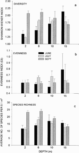
Figure 3. a) Diversity (Shannon-Wiener index), b) evenness expressed by Hill's modified ratio E5, and c) species richness as average number of species per 0.1 m2. (In June n=3, in July and September n=4).

Figure 4. Multi dimensional scaling (MDS) of the zonation pattern in June, July and September. Each point represents one replicate and one depth.

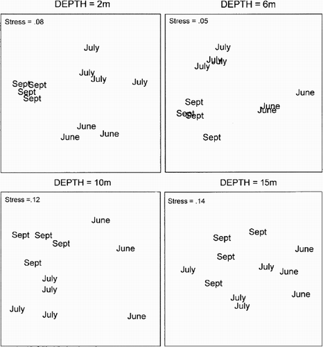
Figure 4. Multi dimensional scaling (MDS) of the zonation pattern in June, July and September. Each point represents one replicate and one depth.
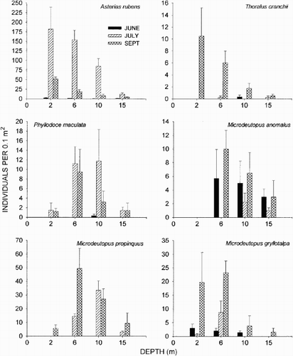
Table III. SIMPER results: the three species that contributed the most (as a percentage) to the total dissimilarity between depths where significant (<0.05) differences occurred. Species depth preference (highest abundance) is also presented.

Figure 5. Multi dimensional scaling (MDS) ordination of temporal variation. Each point represents one replicate and one sampling occasion at the different depths.

Figure 5. Multi dimensional scaling (MDS) ordination of temporal variation. Each point represents one replicate and one sampling occasion at the different depths.

Figure 6. Abundance (individuals per 0.1 m2) of the species responsible for the main (>6%) temporal variation according to the SIMPER analyses. The error bars represent+standard error values.

Figure 6. Abundance (individuals per 0.1 m2) of the species responsible for the main (>6%) temporal variation according to the SIMPER analyses. The error bars represent+standard error values.

Reprints and Corporate Permissions

Please note: Selecting permissions does not provide access to the full text of the article, please see our help page How do I view content?

To request a reprint or corporate permissions for this article, please click on the relevant link below:

Academic Permissions

Please note: Selecting permissions does not provide access to the full text of the article, please see our help page How do I view content?

Obtain permissions instantly via Rightslink by clicking on the button below:

If you are unable to obtain permissions via Rightslink, please complete and submit this Permissions form. For more information, please visit our Permissions help page.