Creating functionally graded concrete materials with varying 3D printing parameters

Figures & data

Figure 1. 3D printed reinforced concrete beam (Asprone et al. 2018).

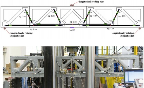
Figure 2. Radial and linear density gradient of concrete samples (Oxman, Keating, and Tsai 2011).

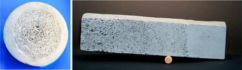
Figure 3. Compacting method to create a linear graded concrete (Gan, Aylie, and Pratama 2015).

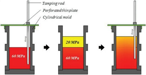
Figure 4. (a) 8 × 3 Periodic lattice topology optimisation design (b) 12 × 3 Periodic lattice topology optimisation design (Rashid et al. 2018).

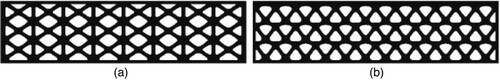
Figure 5. Load vs. displacement graph (Rashid et al. 2018).

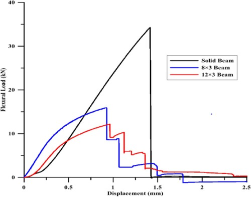
Figure 6. Functionally graded material with different material compositions (Leu et al. 2012).

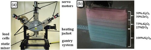
Figure 7. 3D printing for FGCM for; (a) varying fibre deposition systems (Ahmed et al. 2020); (b) multi-material, especially for cock aggregates (Craveiro et al. 2020).

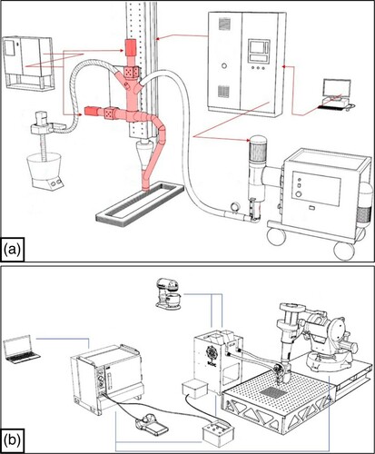
Figure 8. (a) Cumulative percentage passing of raw material (b) Individual percentage retained of raw material.

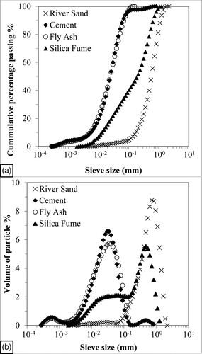
Table 1. Chemical composition (%) of fly ash, silica fume and cement.

Component	SiO2	Al2O3	CaO	Fe2O3	MgO	SO3
Cement	19.7	4.8	63.1	3.2	2.1	2.5
Silica fume	98.4	0.2	0.4	0.1	0.2	0.2
Fly ash	49.2–51.1	28.8–39.4	3.0–5.8	3.5–6.4	0.4–1.1	1.0–1.2

Figure 9. S-shaped printing test print path.

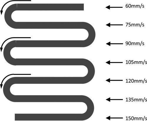
Figure 10. The top view of a schematic drawing of the acceleration-deceleration test print path.

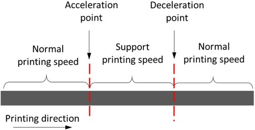
Figure 11. (a) A MBB beam problem with the initial design dimensions (b) Centre-point loading method set-up.

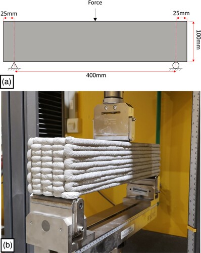
Figure 12. The STL file and slicing preview in slicing software.

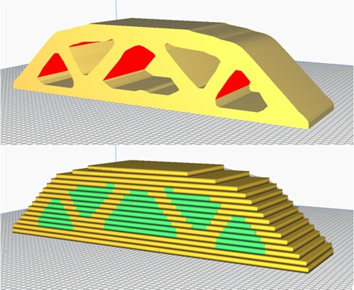
Figure 13. (a) The slicing preview of the 10th layers. (b) The top view of the 10th layer showing the solid and support regions (c) The longitudinal printing path for the 10th layer generated from extracted boundary coordinates with slowed down nozzle travel speed for some of the sections.

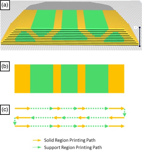
Figure 14. S-shaped printing with round nozzle (a) 6 ml/s (b) 12 ml/s (c) 22 ml/s.

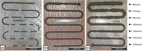
Figure 15. Contour plot of the R_m/i.

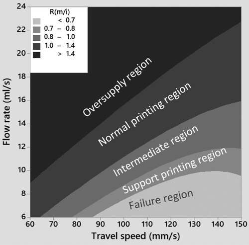
Table 2. R_m/i of filament obtained from ImageJ.

	60 mm/s	75 mm/s	90 mm/s	105 mm/s	120 mm/s	135 mm/s	150 mm/s
24 ml/s	3.49	2.91	2.46	2.08	1.89	1.63	1.52
22 ml/s	3.20	2.64	2.24	1.93	1.74	1.49	1.44
19 ml/s	2.44	2.17	1.80	1.52	1.35	1.19	1.13
16 ml/s	2.19	1.86	1.49	1.36	1.18	1.08	1.00
12 ml/s	1.87	1.44	1.26	1.07	0.97	0.83	0.78
9 ml/s	1.39	1.29	1.02	0.92	0.84	0.79	0.75
6 ml/s	1.00	0.74	0.61	0.52	0.46	0.40	0.39

Figure 16. (a) Ideal travel speed profile of the nozzle (b) Travel speed profile of the nozzle without modification (c) Travel speed profile of the nozzle with modification.

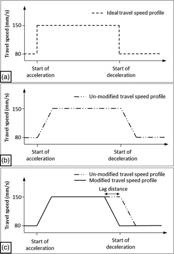
Figure 17. Acceleration-deceleration printing test.

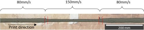
Table 3. Mesh size and total element analysis.

Mesh size (mm)	Total elements	S, Max in plane stress (Mpa)
20	110	1.80248
15	210	1.80019
10	460	1.80048
5	1800	1.80034
3	4950	1.80035

Figure 18. 2D optimised beam structure for the volume-fraction of (a) 20% (b) 40% (c) 60% (d) 80%.

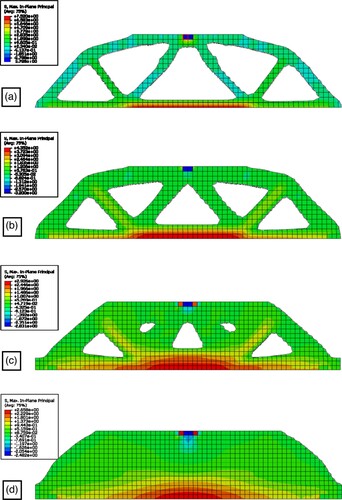
Figure 19. Maximum stress of a 2D optimised structure at different volume constraints.

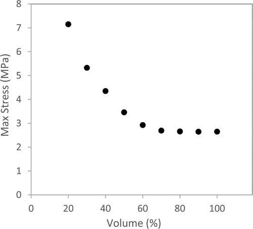
Figure 20. 3D printed structure in the longitudinal direction with a volume-fraction of 100% (b) 80% (c1) a 2D optimised structure of 60% (c2) a 2D optimised structure of 60% with the outline of the strut.

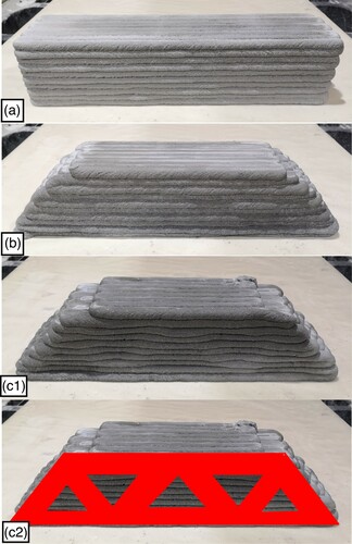
Figure 21. Photo of tested samples (a) 100C (b) 100P (c) 80P (d) 60P.

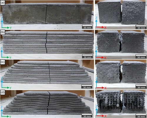
Figure 22. Diagonal view of the 60P sample.

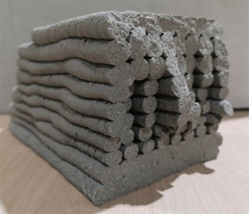
Figure 23. Flexural strength, weight and the strength-to-weight ratio of different samples.

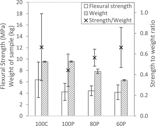
Table 4. Estimated printing time and material used with respective savings for the different samples.

Samples	Printing time	Time saved (%)	Material used (kg)	Std. deviation	Material saved (%)	Std. deviation
60P	301s (5 mins 1 s)	36.5	6.29	0.12	34.36	1.22
80P	407s (6 mins 47 s)	14.1	7.85	0.39	18.06	4.07
100P	474s (7 mins 54 s)		9.58	0.10

Asprone, D., F. Auricchio, C. Menna, and V. Mercuri. 2018. “3D Printing of Reinforced Concrete Elements: Technology and Design Approach.” Construction and Building Materials 165: 218–231. doi:https://doi.org/10.1016/j.conbuildmat.2018.01.018.

 Web of Science ®Google Scholar

Oxman, N., S. Keating, and E. Tsai. 2011. Functionally Graded Rapid Prototyping,” Proceedings of VRAP: Advanced Research in Virtual and Rapid Prototyping, 483–489. doi:https://doi.org/10.1201/b11341-78.

 Google Scholar

Gan, B. S., H. Aylie, and M. M. A. Pratama. 2015. “The Behavior of Graded Concrete, an Experimental Study.” Procedia Engineering 125: 885–891. doi:https://doi.org/10.1016/j.proeng.2015.11.076.

 Google Scholar

Rashid, R., S. H. Masooda, D. Ruan, S. Palanisamy, X. Huang, and R. A. R. Rashid. 2018. “Topology Optimisation of Additively Manufactured Lattice Beams for Three-Point Bending Test.” Annual International Solid Freeform Fabrication Symposium, 635–647.

 Google Scholar

Leu, M. C., B. K. Deuser, L. Tang, R. G. Landers, G. E. Hilmas, and J. L. Watts. 2012. “Freeze-Form Extrusion Fabrication of Functionally Graded Materials.” CIRP Annals 61 (1): 223–226. doi:https://doi.org/10.1016/j.cirp.2012.03.050.

 Web of Science ®Google Scholar

Ahmed, Z. Y., F. P. Bos, M. C. A. J. van Brunschot, and T. A. M. Salet. 2020. “On-Demand Additive Manufacturing of Functionally Graded Concrete.” Virtual and Physical Prototyping 15 (2): 194–210. doi:https://doi.org/10.1080/17452759.2019.1709009.

 Web of Science ®Google Scholar

Craveiro, F., S. Nazarian, H. Bartolo, P. J. Bartolo, and J. Pinto Duarte. 2020. “An Automated System for 3D Printing Functionally Graded Concrete-Based Materials.” Additive Manufacturing 33: 101146. doi:https://doi.org/10.1016/j.addma.2020.101146.

 Web of Science ®Google Scholar