Acoustic feature based geometric defect identification in wire arc additive manufacturing

Figures & data

Table 1. Prior work concerning acoustic defect detection in metal AM.

AM process	Targeted Defects	Limitations
	Balling, Micro defects,	No geometric defect detection
LPBF, LDED,	Lack of fusion pores,
PBF, SLM	Keyhole pores, Crack,
	Porosity
WAAM	Line width variation,
	Voids,	Not classify specific defects
	Porosity,	Not scalable to other defects
	Spatter

Figure 1. Schematic representation of a multi-beads printing (left) and Actual printing (right) as seen from the build direction. Geometrically defective segments lead to voids between two successive beads will affect the final printed part strength and quality.

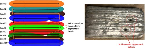
Figure 2. The methodology for constructing the geometric defect detection Frameworks.

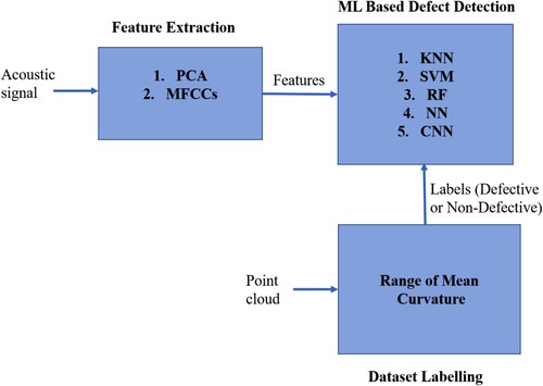
Figure 3. Experimental setup of SUTD Robotic WAAM for Bead Geometry and Acoustic Data Collection (left). (a) Original beads with plate (b) Mesh representation of beads with plate (right).

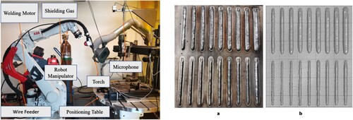
Figure 4. DFT features of a segmented signal (left) MFCC features of a segmented signal (right).

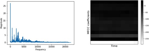
Figure 5. Range of mean curvature of geometrically good (left) and bad (right) bead segment. The red circle indicates a geometric defect.

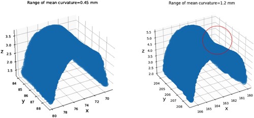
Figure 6. Bead with defective and non-defective segments (Top) with corresponding acoustic time-domain waveforms (Middle) and range curvature (Bottom).

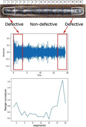
Figure 7. The proposed NN Architecture for defective bead segments identification.

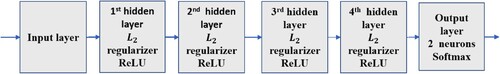
Figure 8. The proposed CNN Architecture for defective bead segments identification.

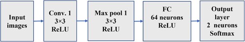
Figure 9. Distribution plots for good and bad segments of beads for different thresholds (First three plots). Different thresholds vs overlapping area plot(last plot).

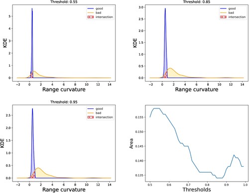
Figure 10. KNN classification error based on the number of nearest neighbour K and weight function for PCA features (top plot) and MFCC features (bottom plot).

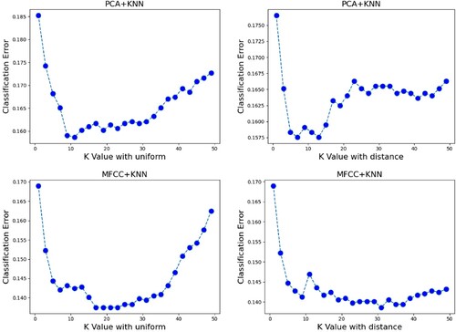
Figure 11. SVM classification error based on the choice of γ and C for the RBF and Sigmoid kernels with PCA features (top) and MFCC features (bottom).

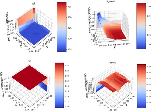
Figure 12. RF classification error based on the number of trees for PCA features (left plot) and MFCC features (right plot).

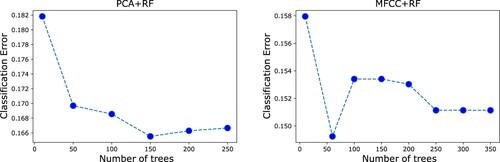
Figure 13. NN Classification accuracy based on the number of layers of a NN architecture for PCA features (left plot) and MFCC features (right plot).

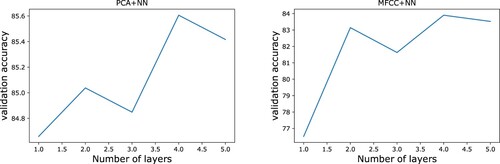
Table 2. Different Combination of number of neurons for PCA+NN.

layer 1	layer 2	layer 3	layer 4	validation accuracy
256	128	64	32	84.1
192	128	64	32	83.6
128	128	64	32	83.1
256	82	64	32	83.9
256	100	64	32	84.2
256	128	64	32	84.4
256	128	64	32	84.5
256	128	56	32	83.6
256	128	48	32	83.5
256	128	64	32	84.1
256	128	64	24	83.06
256	128	64	16	82.59

Table 3. Different Combination of number of neurons for MFCC+NN.

layer 1	layer 2	layer 3	layer 4	validation accuracy
256	128	64	16	83.7
192	128	64	16	83.5
128	128	64	16	83.2
256	82	64	16	83.4
256	100	64	16	83.6
256	128	64	16	82.8
256	128	64	16	83
256	128	56	16	82.4
256	128	48	16	82.1
256	128	64	32	81.8
256	128	64	24	82.2
256	128	64	16	82.9

Figure 14. CNN classification accuracy based on the number of filters within its architecture for PCA features (left plot) and MFCC features (right plot).

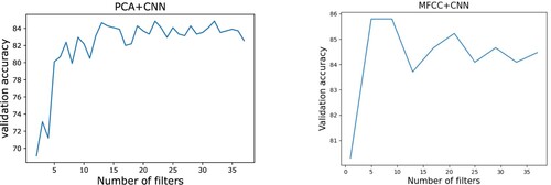
Figure 15. Average validation accuracy for the different defect identification models vs the number of principal components used as a feature.

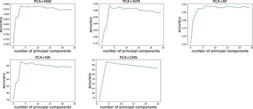
Figure 16. The loss curve for PCA+NN and MFCC+NN (top) The loss curve for PCA+CNN and MFCC+CNN (bottom).

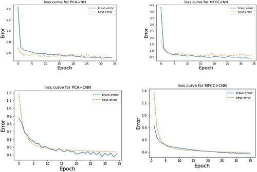
Table 4. Comparative study of all of the proposed defect identification model based on F1 score, precision, and recall.

Defect Identification Model	F1 Score	Precision	Recall
PCA+KNN	$80.59\pm 0.05$	$81.86\pm 0.03$	$80.06\pm 0.11$
PCA+SVM	$83.50\pm 0.08$	$87.06\pm 0.08$	$81.29\pm 0.06$
PCA+RF	$80.71\pm 0.04$	$81.18\pm 0.03$	$80.21\pm 0.11$
PCA+NN	$82.80\pm 0.03$	$84.41\pm 0.08$	$82.11\pm 0.05$
PCA+CNN	$82.26\pm 0.06$	$84.63\pm 0.03$	$80.01\pm 0.05$
MFCC+KNN	$83.19\pm 0.08$	$87.15\pm 0.06$	$81.62\pm 0.07$
MFCC+SVM	$84.24\pm 0.08$	$88.65\pm 0.06$	$82.65\pm 0.01$
MFCC+RF	$84.18\pm 0.03$	$87.28\pm 0.03$	$82.10\pm 0.07$
MFCC+NN	$81.21\pm 0.17$	$82.44\pm 0.05$	$80.67\pm 0.02$
MFCC+CNN	$79.45\pm 0.07$	$82.55\pm 0.08$	$77.44\pm 0.11$

Table 5. Comparative study of all of the proposed defect identification model based on Confusion Matrix.

Defect Identification Model	True
			Good	Bad
PCA+KNN	Predicted	Good	354	59
		Bad	61	186
PCA+SVM	Predicted	Good	400	83
		Bad	15	162
PCA+RF	Predicted	Good	366	68
		Bad	49	177
PCA+NN	Predicted	Good	381	68
		Bad	34	177
PCA+CNN	Predicted	Good	388	77
		Bad	27	168
MFCC+KNN	Predicted	Good	393	75
		Bad	22	170
MFCC+SVM	Predicted	Good	405	80
		Bad	10	165
MFCC+RF	Predicted	Good	395	73
		Bad	20	172
MFCC+NN	Predicted	Good	369	76
		Bad	46	169
MFCC+CNN	Predicted	Good	399	77
		Bad	16	168