Figures & data
Figure 1. (a) Large-scale AM system featuring an articulated robotic arm and a viscous materials dispenser printing a large-scale prototype. (b) Process control parameters include the motion velocity v, flow of material extrusion f, spacing between layers z, and nozzle diameter d.
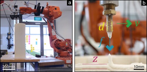
Figure 2. Examples of 3D printed surfaces with 120 mm diameter at the base and 10, 20, and 30 layers with −10, 0, and +10 degrees of taper angle from the vertical direction.
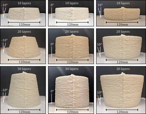
Figure 3. (a) Structured-light 3D scanning equipment acquiring cylindrical specimens. (b) Details of resulting mesh geometry generated. (c) Registration procedure steps.
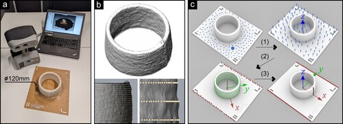
Figure 4. Neural network configurations (a) trained and (b) evaluated, including the Pareto frontier between loss and number of trainable parameters. The smallest network uses one hidden layer of 32 neurons, while the largest contains three layers of 3072 neurons.
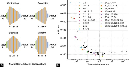
Figure 5. Approximation characteristics of a simple (one layer with 32 neurons) and a complex (three layers of 128, 64, and 32 neurons) network predicting (a) the radial deformation and (b) residuals for a cylinder with 25 layers and 100 mm diameter at its 10-th layer. (c) Correction scheme iterations versus loss and (d) MSE error map for a 20-layer 100 mm diameter cylinder using the (128, 64, 32) network.
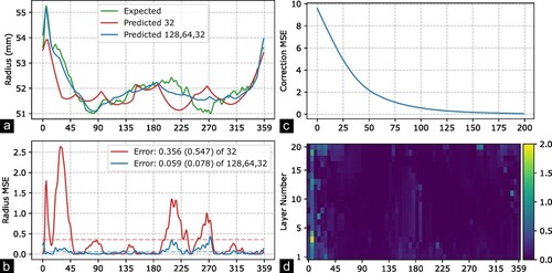
Figure 6. (a) Wet and (b) dry states of a 100 mm diameter, 20-layer cylinder, including (c) overlays of photography and (d) section view of the acquired meshes, highlighting visually the effects of shrinkage resulting in significant geometric deformation.
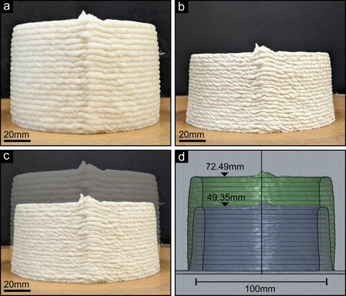
Figure 7. (a) Dry-to-wet mass ratio of a 100 mm diameter, 20-layer cylindrical prototype, using a 7 mm nozzle diameter, under various drying regimes. The dotted line represents normalisation to room temperature and humidity. (b) Vertical shrinkage per number of layers including both cylinders and cones of various taper angles.
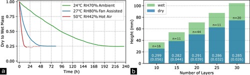
Figure 8. (a) Wet and dry filament perimeter lengths for a 100 mm diameter, 20-layer cylinder, and longitudinal shrinkage per layer. (b) Wet and dry filament run widths for the same cylinder and transverse shrinkage per layer.
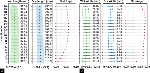
Figure 9. Comparison of uncorrected and corrected 20-layer cylinders with 100 mm diameter. (a) Section view of profiles and distribution of errors. (b) Polar graph depicting the same cylinder in plan view.
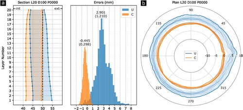
Figure 10. Isometric view of (a) uncorrected and (b) corrected cylinders with 20 layers and 100 mm diameter showing the relative errors from the mean base radius and distributions thereof.
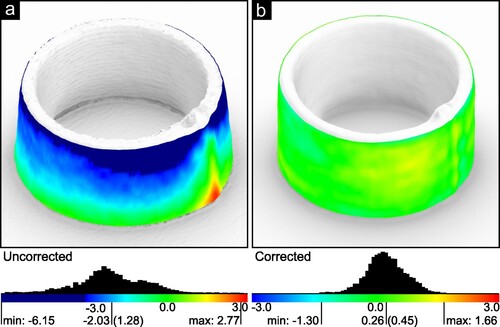
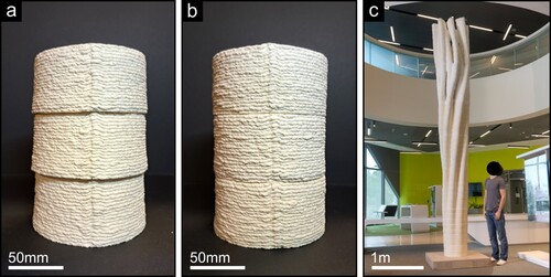
Figure 11. (a) Uncorrected and (b) corrected cylinders with 20 layers and 100 mm diameter stacked vertically. (c) Example of a large-scale 3D print design measuring 5 m tall, comprised of 50 segments.