Numerical modelling of the viscoelastic polymer melt flow in material extrusion additive manufacturing

Figures & data

Figure 1. (a) Schematic of FDM process; (b) Geometry of the hot-end channel and boundary conditions of the computational model.

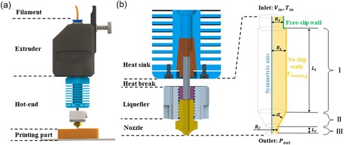
Table 1. Dimensions of INTAMSYS HT400 hot-end.

Dimension	Symbol	Value	Unit
Filament radius	${\mathit{R}}_{\mathit{F}}$	0.875	mm
Liquefier radius	${\mathit{R}}_{\mathit{L}}$	1	mm
Nozzle radius	${\mathit{R}}_{\mathit{C}}$	0.2	mm
Capillary length	${\mathit{L}}_{\mathit{C}}$	0.6	mm
Liquefier length	${\mathit{L}}_{\mathit{L}}$	20	mm
Contraction angle	$\mathit{\alpha }$	30	${}^{\circ }$

Figure 2. (a) Fitted curve for storage and loss moduli $G^{\mathrm{\prime }}$ and ${\mathrm{G}}^{\mathrm{\prime \prime }}$. (b) Fitted curve for viscosity.

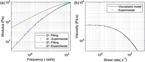
Table 2. Identified parameters for the constitutive model.

Viscoelastic Model
Parameter	Symbol	Unit	Value
			Mode 1	Mode 2	Mode 3
Mobility factor	${\alpha }_k$	–	0.609	0.794	0.485
Relaxation time	${\lambda }_{k0}$	$S$	0.0048	0.265	0.0249
Polymer viscosity contribution	${\eta }_{k0}$	$\mathrm{Pa}\cdot s$	615.1	965.4	987.1
Solvent viscosity contribution	${\eta }_{s0}$	$\mathrm{Pa}\cdot s$	131.4
GNF Model
Zero-shear viscosity	${\eta }_o$	$\mathrm{Pa}\cdot s$	2011.5
Relaxation time	${\lambda }^{\ast }$	$S$	0.014
Power-law index	$n$	–	0.26
Arrhenius Equation
Reference temperature	$T_0$	$K$	453.2
Activation energy/Gas constant	$\mathrm{\Delta H}/R_{\mathrm{ig}}$	$K$	10880

Table 3. Material properties adopted in the simulation.

Parameter	Symbol	Value	Unit	Source
Density	$\rho$	1.18	$g/c{m}^3$	[33]
Thermal conductivity	$\kappa$	0.2	$W/\mathrm{mK}$	[9]
Melting enthalpy	$L$	100	$J/g$	[9]
Solidus melting temperature	$T_s$	413.15	$K$	[9]
Liquidus melting temperature	$T_l$	428.15	$K$	[9]
Glass temperature	$T_g$	334.15	$K$	[33]

Figure 3. Measured and predicted feeding force at different feeding rates. The predictions are conducted for various $A_{\mathrm{mush}}$ and generated using two models: (a) the GNF model and (b) the viscoelastic model.

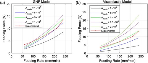
Figure 4. Influence of different $A_{\mathrm{mush}}$ on the simulation results for the liquid phase fraction and temperature distribution at different $A_{\mathrm{mush}}$.

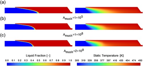
Figure 5. Prediction of transient feeding force under the isothermal flow assumption.

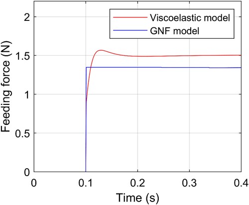
Figure 6. Feeding force response with the GNF model (c) and viscoelastic model (e) under the step velocity input (a). Feeding force response with the GNF model (d) and viscoelastic model (f) under the trapezoidal velocity profile (b).

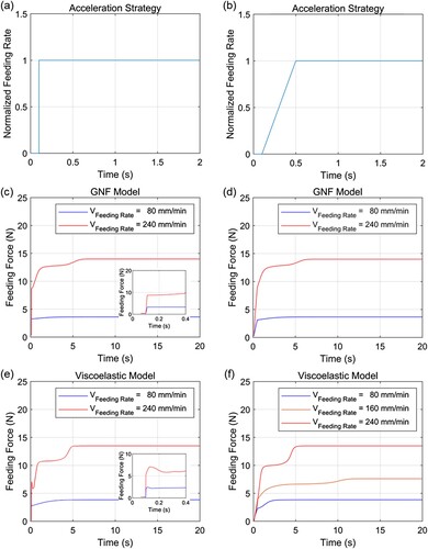
Figure 7. Distribution for solid-liquid phase, streamline and each component of the stress tensor at a feeding rate of 60 mm/min.

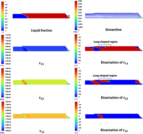
Figure 8. Comparison of distribution for normal stress difference $N_1$ and shear stress ${\tau }_{12}$ at different feeding rates.

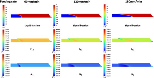
Figure 9. Curves about the area integral at the outlet for the normal stress difference and each stress tensor component versus the feeding rate.

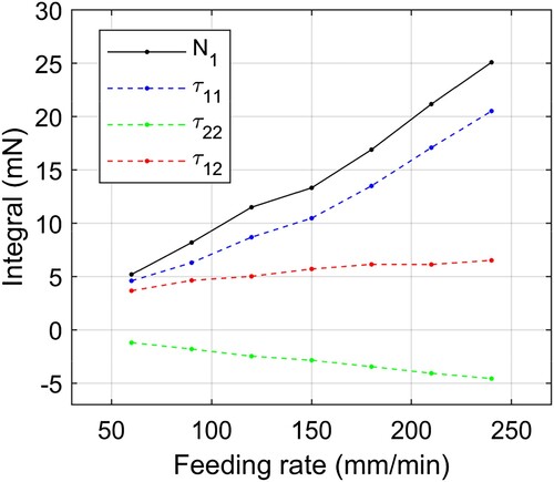
Figure A1. Experiment setup of feeding force measurement instrument.

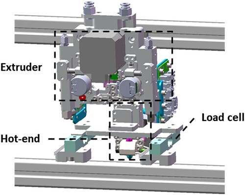
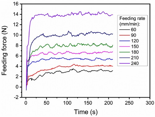
Figure A2. Experimental data curves of feeding force at different feeding rates.

Polymaker. (2019). “PolyLiteTM PLA.” https://us.polymaker.com/products/polylite-pla%0Ahttps://polymaker.com/product/polylite-pla/.

 Google Scholar

Phan DD, Horner JS, Swain ZR, et al. Computational fluid dynamics simulation of the melting process in the fused filament fabrication additive manufacturing technique. Add Manuf. 2020;33(May). doi:10.1016/j.addma.2020.101161

 Google Scholar

Data availability statement

The data that support the findings of this study are available from the corresponding author, [YX], upon reasonable request.