
Figures & data
Figure 1. (a) SGMP configuration; (b) MG configuration. (c,d) An example of the PAD configuration (10) (c) robotic arms placements (c) and (d) printing areas.
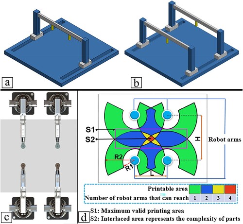
Figure 2. Single and cooperative printing areas for (a) MG configuration; (b) PAD configuration. (c) MA configuration.
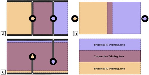
Figure 3. Three MA configurations with a different number of printheads (a) two printheads (b) four printhead, and (c) five printheads.
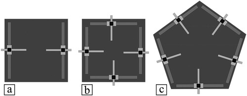
Figure 4. (a) Developed MA cooperative printing system; (b) detailed CAD model of the MA gantry system (belts and cables are not shown).
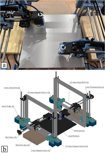
Figure 5. The cooperative and noncooperative safety areas of the machine. Dimensions are in mm.
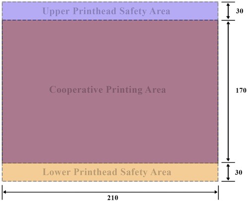
Figure 6. The T-bot mechanism that allows arm extension.
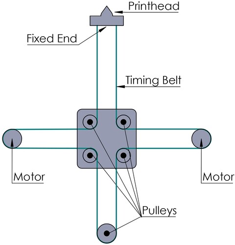
Figure 7. Information flow in the developed path planner.
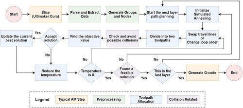
Figure 8. Grouping method: (a) no groups, (b) few groups, (c) a large number of groups. Loops breakage: (d) include all loops, (e) break all loops (f) break inner loops only.
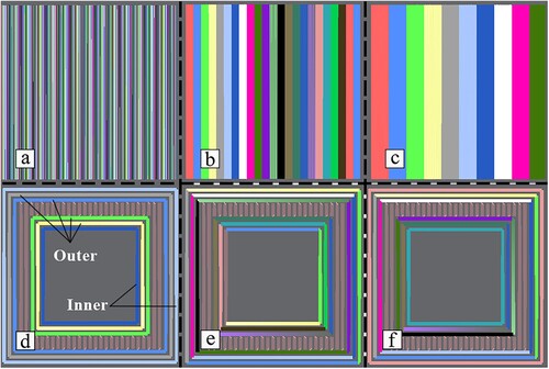
Figure 9. Examples of (a) the planner visiting a loop, and (b) the planner deciding which node to travel to from node 1. The green point is the current point for the planner.
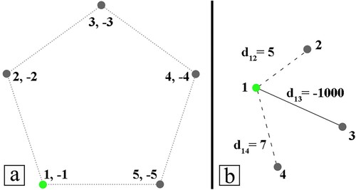
Figure 10. Different algorithms to locally modify the original path: (a) original toolpaths; (b) travel paths modifications; (c) loop order changes; (d) final result.
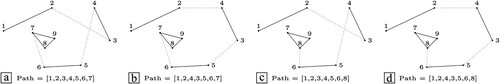
Figure 11. Two situations for collision avoidance, (a) a situation that can be avoided by delay-based methods; (b) a situation that cannot be avoided by delay-based methods.
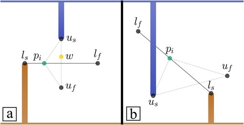
Figure 12. Visualisation of the shifting method. (a) Starting of the motion showing the shifted lower printhead in faded orange; (b) the upper printhead touches the shifted lower printhead at the intermediate point.
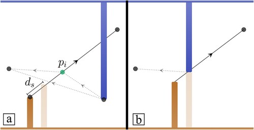
Figure 13. The randomised simulation procedure used to compare the performance of both IPM and DBM.
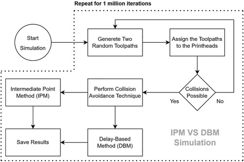
Table 1. Comparison of the IPM with DBM for collision avoidance.
Figure 14. IPM generation of multiple points. (a–d) The motion of the two printheads doing several print and travel lines; (e) the swept area of the upper printhead toolpath and the area of the lower printhead at the starting position.
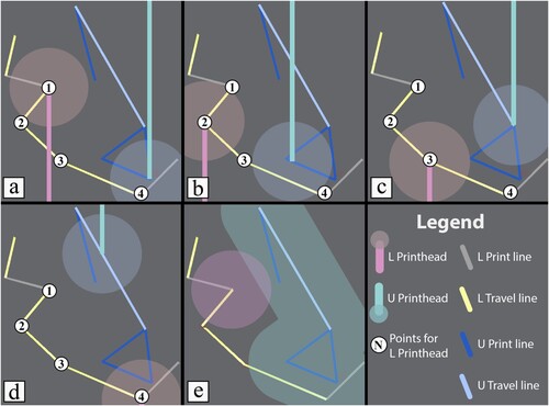
Figure 15. Problematic model and the specific problematic layer for (a) SGMP, (b) PAD, and (c) MG configurations. The right side shows how the MA configuration solves each problematic layer efficiently. The blue and grey regions correspond to the upper and lower printheads, respectively.
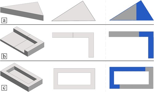
Figure 16. Effect of rectilinear pattern angles on both computation time and printing time reduction.
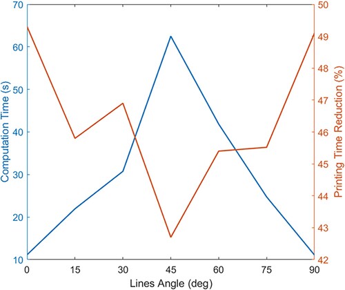
Figure 17. A single layer at four distinct angles: (a) 0°, (b) 90°, (c) 180°, (d) and 270°. Top: the generated toolpaths, Bottom: the groups generated from the grouping method.
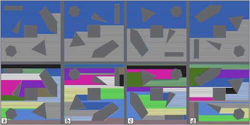
Figure 18. The three different objects with layers tested for cooperative printing using the developed algorithms. (a) Topology optimised bracket (38), (b) nose of a wind turbine (39), and (c) wing of an airplane (40). The top images show the CAD models and the bottom images correspond to sample layers from the models where the system has generated toolpaths for two printheads. Blue and grey regions correspond to the upper and lower printheads, respectively.
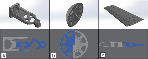
Figure 19. The three different layers tested for cooperative printing using the developed system. (a) A model of each layer and (b) the generated toolpaths for two printheads MA system. In (b), blue and grey regions correspond to the upper and lower printheads, respectively.
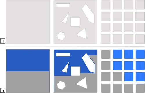
Figure 20. Cooperative printing of three different single-layer objects.
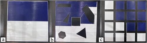
Figure 21. Toolpaths of the (a) lower and (b) upper arms, and (c) the printed object.
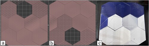
Figure 22. Images of the machine printing the hexagonally tiled object. The full video is available at: https://youtu.be/mrDgoHUAMtE?si = fGEjtKyiKE2E-yTW.
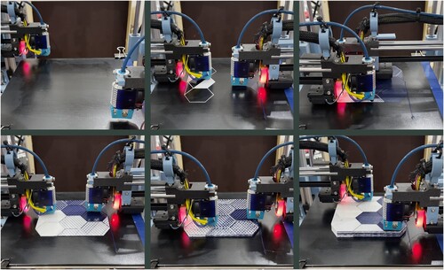
Figure 23. An object with distant features. (a) Single-print head toolpath (blue lines are the travel lines), and (b) 3D printed part with the developed machine.
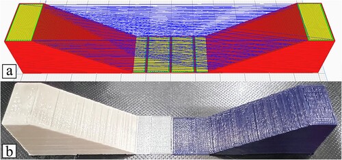
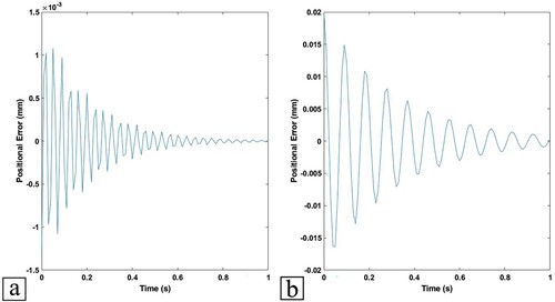
Figure 24. The effect of vibrations on the position of the printhead. (a) The effect at 10 mm on the Y-axis; (b) the effect at 200 mm on the Y-axis.
Data availability statement
The data that support the findings of this study are available from the corresponding author upon reasonable request.