Modelling, optimization, and testing of novel cuboidal spherical plate lattice structures

Figures & data

Figure 1. The procedure of generating the CSPL unit cells, showing: (a) CSPL 111, (b) CSPL 111 + 100, and (c) CSPL 111 + 110.

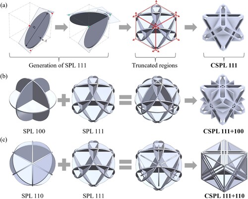
Figure 2. Demonstrating the correlation between the relative density and the aspect ratio for the CSPLs: (a) linear correlation between $\overline{\rho }$ and t/D, and (b) illustrating cross-sections from the top view of the designs at different $\overline{\rho }$ and t/D.

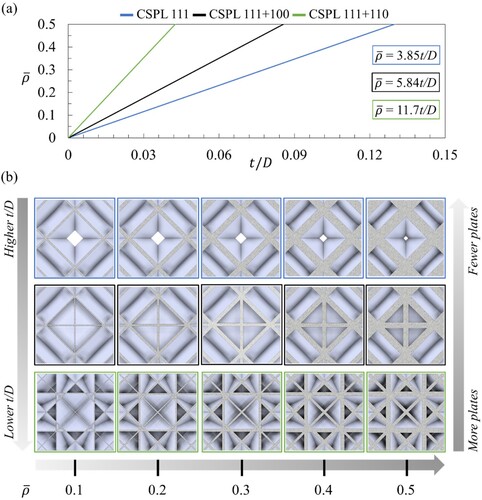
Figure 3. (a) 3D model of CSPL 111 + 110 deomstrating the normal and the shearing stresses, and (b) mesh sensitivity analysis for the CSPLs at different relative densities.

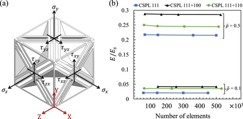
Figure 4. Normalised effective elastic properties of the CSPLs, (b) uniaxial modulus, (c) shear modulus and (d) bulk modulus.

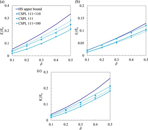
Figure 5. Mises stress distribution in CSPLs with $\overline{\rho }$ = 0.4 for various loading conditions: (a) uniaxial, (b) shear and (b) hydrostatic loading.

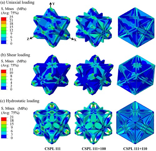
Table 1. A summary of the scaling law parameters of the elastic moduli of the CSPLs.

	$E/E_s$		$G/E_s$		$K/E_s$
	$C$	$n$	$C$	$n$	$C$	$n$
CSPL 111	0.58	1.46	0.25	1.25	0.49	1.45
CSPL 111 + 100	0.63	1.18	0.23	1.23	0.46	1.23
CSPL 111 + 110	0.56	1.19	0.26	1.10	0.49	1.21

Figure 6. Demonstrating the deformation modes of the CSPLs under (a) uniaxial, (b) shear, and (c) hydrostatic loading for the case of $\overline{\rho }$ = 0.4.

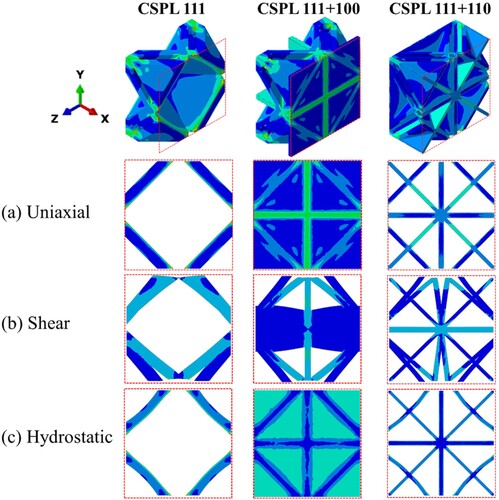
Figure 7. Uniaxial and shear moduli distributions of CSPLs with $\overline{\rho }$ = 0.4.

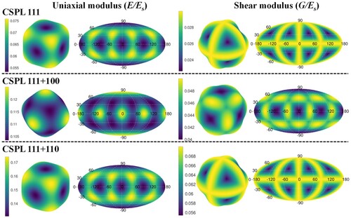
Figure 8. Elastic parameters for CSPLs: (a) effective Poisson’s ratio $v$, (b) Zener’s index A for and (c) total stiffness $\mathrm{\Omega }$.

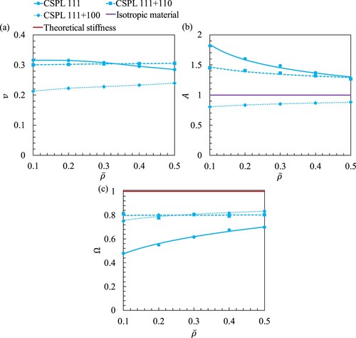
Figure 9. Effective stress-strain curves for (a) CSPL 111, (b) CSPL 111 + 100, (c) CSPL 111 + 110, and normalised effective yielding properties: (d) uniaxial yiled strength, (e) shaer yield strength and (f) hydrostatic yield strength.

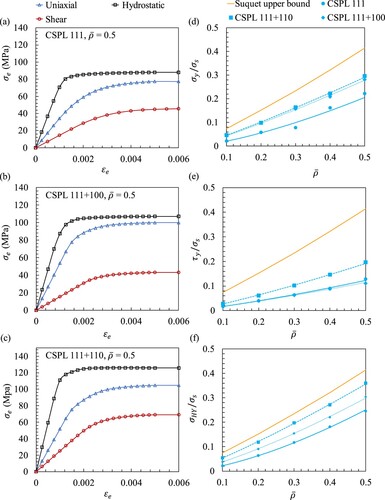
Table 2. A summary of the scaling law parameters of the yield strengths for the CSPLs.

	${\sigma }_y/{\sigma }_s$		${\tau }_y/{\sigma }_s$		${\sigma }_{\mathrm{HY}}/{\sigma }_s$
	$C$	$n$	$C$	$n$	$C$	$n$
CSPL 111	0.55	1.42	0.71	1.51	0.29	1.23
CSPL 111 + 100	0.62	1.16	0.73	1.29	0.26	1.19
CSPL 111 + 110	0.64	1.14	0.80	1.18	0.44	1.20

Figure 10. The constrained-domain topoloy optimisation procedure for CSPL 111 + 110, showing: (a) applied loading and boundary condition, (b) compliance minimisation throughout the simulation, (c) the raw output of 1/8th of TOCSPL 111 + 110, and (d) the postprocessed output of the complete unit cell of TOCSPL 111 + 110.

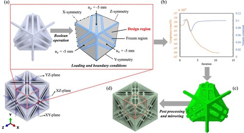
Figure 11. (a) Post-processed topology optimised TOCSPLs at different final relative densities. (b) a few examples demonstrating the benefit of the constrained-domain topology optimisation, such as, filling opened surfaces and smoothening sharp edges. (c) a few examples demonstrating the cross-sectional views of the TOCSPLs.

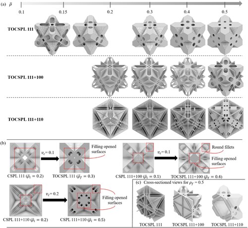
Table 3. A summary of the required initial relative densities and volume constraints to produce the corresponding topologically optimised CSPLs.

Structure	${\rho }_i$	$V_c$	${\rho }_f$
CSPL 111	0.05	0.05	0.145
	0.05	0.1	0.186
	0.2	0.1	0.3
	0.3	0.1	0.4
	0.4	0.1	0.5
CSPL 111 + 100	0.1	0.05	0.2
	0.2	0.03	0.3
	0.1	0.1	0.4
	0.2	0.1	0.5
CSPL 111 + 110	0.05	0.01	0.225
	0.05	0.1	0.3
	0.1	0.2	0.4
	0.2	0.2	0.5

Figure 12. Effective elastic and yielding properties of the TOCSPLs, compared with other types of lattice materials, showing: (a) uniaxial, (b) shear and (c) bulk moduli, and (d) uniaxial, (e) shear and (f) hydrostatic yield strength.

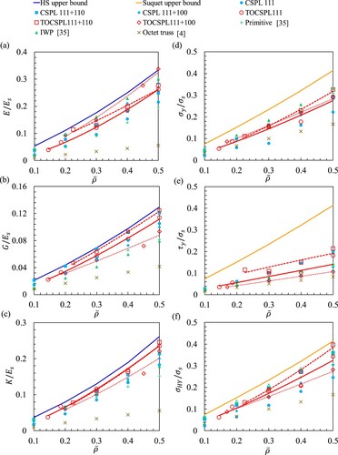
Figure 13. Mises stress distribution of the TOCSPLs with $\overline{\rho }$ = 0.4 as a result of different loading conditions: (a) uniaxial, (b) shear and (c) hydrostatic loading.

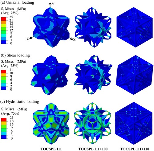
Figure 14. Change in the effective mechanical properties between CSPL and TOCSPL lattices, showing: (a) uniaxial, (b) bulk and (c) shear moduli, and (d) uniaxial, (e) hydrostatic and (f) shear yield strength.

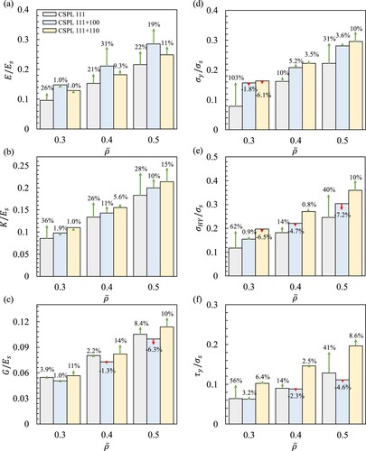
Figure 15. (a) Zener’s index A and (b) the total stiffness Ω of the CSPLs, with their topology optimised counterparts TOCSPLs.

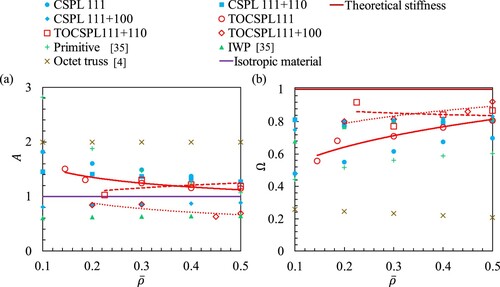
Figure 16. Illustration of the effect of process parameters on the surface roughness and the mechanical strenght of a CSPL 111 + 100 structure: (a) the efffect of layer height on the print duration and layer strenght and (b) the effect of infill density on the print duration.

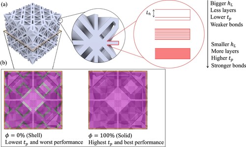
Table 4. A summary of the process parameters utilised in the FDM printer (Sindoh 3D WOX1).

Description	Parameter	Value	Units
Layer height	$h_L$	0.15	mm
Wall thickness	$w_t$	0.8	mm
Nozzle temperature	$T_N$	230	°C
Bed temperature	$T_B$	90	°C
Infill density	$\varphi$	100	%
Print speed	–	35	mm/s
Travel speed	–	130	mm/s

Figure 17. (a) Comparison between the as-designed and the measured relative densities of the additively manufactured samples and (b) additively manufactured samples with $\overline{\rho }$ = 0.5.

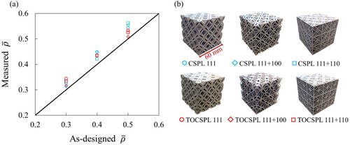
Figure 18. Applying the tangent method based on the stress-strain curves to determine the densification strain ${\epsilon }_d$ of: (a) CSPL 111 + 100 with $\overline{\rho }$ = 0.3, and (b) TOCSPL 111 + 110 with $\overline{\rho }$ = 0.4.

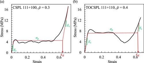
Figure 19. (a) Experimental stress-strain diagrams of the CSPL 111 with $\overline{\rho }$ = 0.3 tested at different number of arrays, (b) snapshots of the deformation patterns at different strains, and showing (c) compressive modulus and (d) SEA.

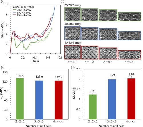
Figure 20. Experimental stress-strain digarms of the CSPLs and the TOCSPLs with different relative densities: (a) CSPL 111 and TOCSPL 111, (b) CSPL 111 + 100 and TOCSPL 111 + 100, (c) CSPL 111 + 110 and TOCSPL 111 + 110. Bar charts representing the mechanical properties of CSPLs and TOCSPLs: (d) compressive modulus, (e) SEA, (f) uniaxial yield strength.

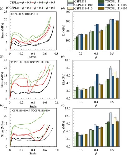
Figure 21. Experimental snapshots and simulation results of quasi-static compression testing for the CSPLs at different strains for the case $\overline{\rho }$ = 0.3.

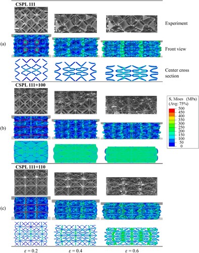
Figure 22. Experimental snapshots and simulation results of quasi-static compression testing for the TOCSPLs at different strains for the case $\overline{\rho }$ = 0.3.

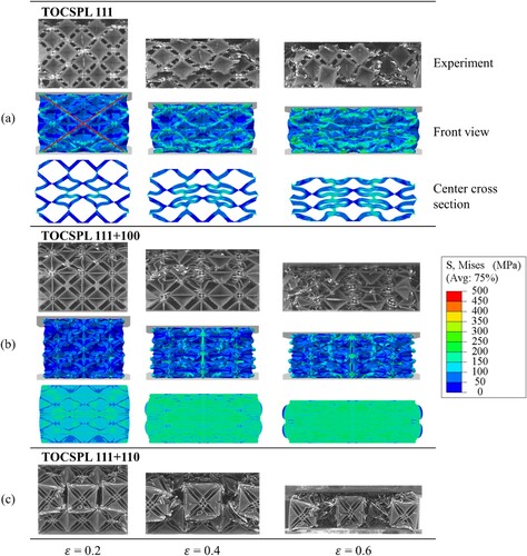
Figure 23. Model for elastic-plastic compression simulations (CSPL 111, $\overline{\rho }$ = 0.3).

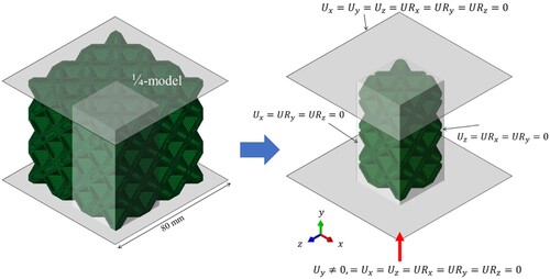
Figure 24. (a) Experimental and numerical stress-strain diagrams of the CSPLs and the TOCSPLs for the case $\overline{\rho }$ = 0.3. Bar charts comparing the experimental and numerical mechanical properties of the CSPLs, showing (b) compressive modulus, (c) uniaxial yield strength, and (d) SEA.

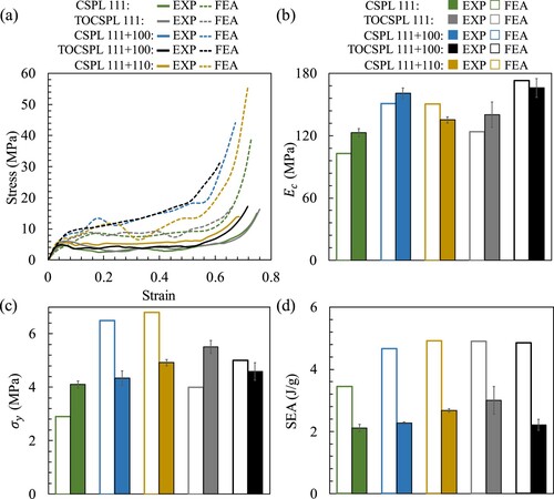
Figure 25. Comparing lattice materials from the literature and designs proposed in this work using experimentally determined normalised elastic modulus.

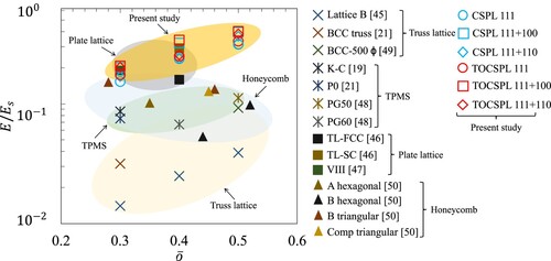
Figure 26. Comparing lattice materials from the literature and designs proposed in this work using experimentally determined normalised yield strength.

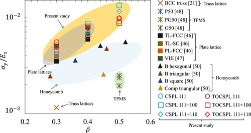
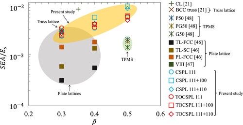
Figure 27. Comparing lattice materials from the literature and designs proposed in this work using experimentally determined normalised energy absorption.

Data availability statement

Data will be made available on request from the authors.