
Figures & data
Figure 1. Staircase effect. (a) Planar layering, (b) adaptive layering and (c) curved layering.
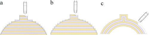
Figure 2. Layering results of typical parts based on voxelization. (a) Logarithmic spiral gear model, (b) submarine shell model, (c) pipe model, (d) logarithmic spiral gear layering result, (e) submarine shell layering result and (f) pipe layering result.
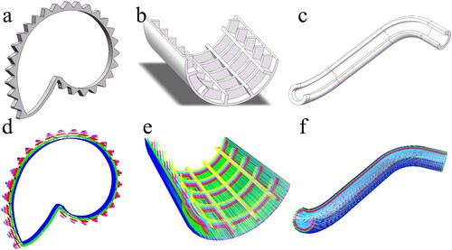
Figure 3. Voxelization procedure. (a) The minimum bounding box of the STL model, (b) model rotating, (c) meshing, (d) calculation of intersection point and (e) voxelization result.
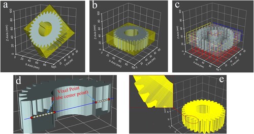
Table 1. Comparison of neighbourhood search operation time with different data structure.
Figure 4. Extended geodesic distance diagram.
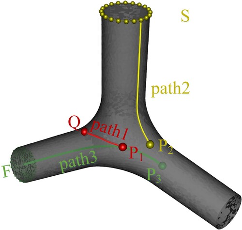
Figure 5. Flow chart of geodesic distance calculation.
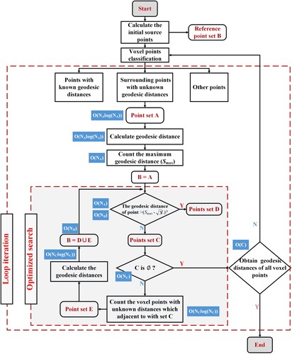
Figure 6. Schematic diagram of voxel point neighbourhood search.
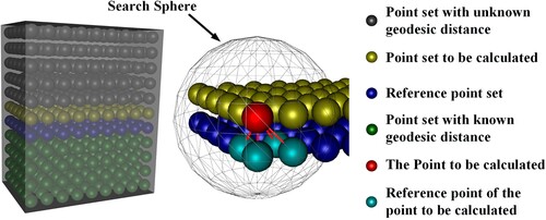
Figure 7. Diagram of geodesic distance deviation.
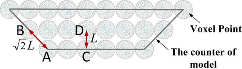
Figure 8. Diagram of proof process.
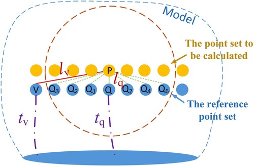
Figure 9. Schematic diagram of geodetic distance calculation process. (a) Calculation process of direct search and (b) calculation process of optimization search.
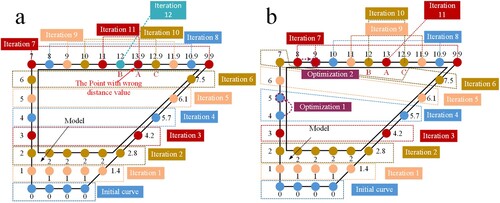
Figure 10. Comparative effects of different curved layering methods.
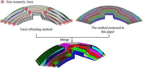
Figure 11. Error analysis of the facet offsetting method in degenerate case. (a) Schematic diagram of degradation situation and (b) error distribution.
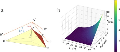
Figure 12. The problem of traditional path planning.
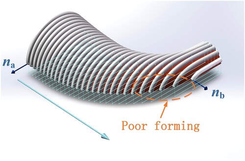
Figure 13. Planning effects from different initial paths.
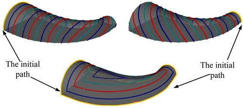
Figure 14. Diagram of the shortest deposition direction and positioner angle planning. (a) The shortest deposition direction in case 1, (b) the shortest deposition direction in case 2, (c) adjust the shortest deposition direction in case 1 and (d) adjust the shortest deposition direction in case 2.
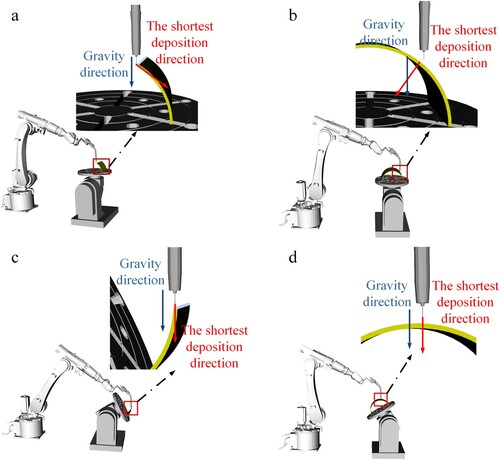
Figure 15. Steps for calculating the joint angle of the positioner. (a) The shortest deposition direction at the initial position; (b) rotating movement and (c) tilting movement.
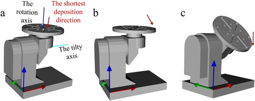
Figure 16. GMA-AM experiment setup. (a) Hardware and (b) software interface.
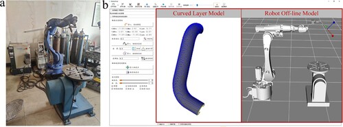
Table 2. Chemical constituents of substrate and wires (wt. %).
Figure 17. Feature dimensions and model of turbine. (a) Feature dimensions and (b) 3D-model.
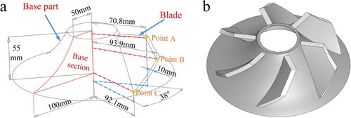
Figure 18. Path planning on turbine base surface.
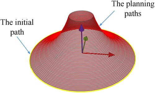
Figure 19. Curved layering and path planning of turbine blade. (a) Curved layering result and (b) path planning result.
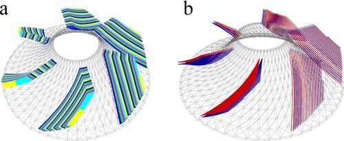
Figure 20. The results of planar layering method. (a) Slicing along the axial direction of the blade and (b) slicing along the normal direction of substrate.
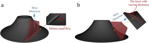
Figure 21. Positioner pose in offline programming simulation environment. (a) Path point 1, (b) path point 2, (c) path point 3 and (d) path point 4.
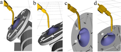
Figure 22. The pose in the real depositing process. (a) Path point 1, (b) path point 2, (c) path point 3 and (d) path point 4.
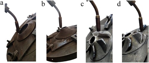
Figure 23. Turbine base planning and depositing process. (a) Path planning result of the first 15 layers, (b) path planning result of the first 30 layers, (c) path planning result of the 54 layers. (d) forming morphology of 15 layers, (e) forming morphology of layer 30 and (f) forming morphology of layer 54.
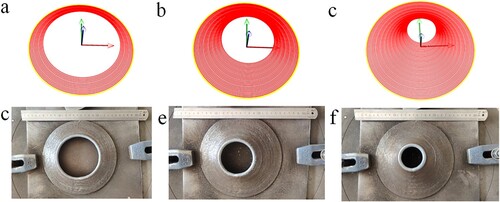
Figure 24. Turbine blade depositing process. (a) Curved layering result of the first layer, (b) curved layering result of the first 10 layers, (c) curved layering result of the 20 layers, (d) Forming morphology of the first layer, (e) forming morphology of the first 10 layers and (f) forming morphology of the 20 layers.
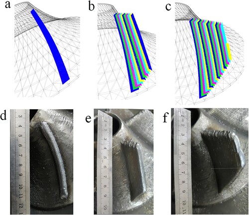
Figure 25. Turbine forming appearance and accuracy. (a) Appearance of finished part, (b) scanned model and (c) error distribution.
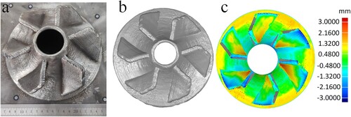
Figure 26. Impeller forming appearance based on planar layering method [Citation32].
![Figure 26. Impeller forming appearance based on planar layering method [Citation32].](/cms/asset/7b391435-ecef-478e-b0c7-a4cc39e24739/nvpp_a_2346289_f0026_oc.jpg)
Data availability statement
The data presented in this study are available on request from the corresponding author.