Inhomogeneity and anisotropy of Al-Zn-Mg-Cu alloy manufactured by wire arc additive manufacturing: microstructure, mechanical properties, stress corrosion cracking susceptibility

Figures & data

Figure 1. (a) WAAM system, (b) Schematic diagram of welding torch and working platform, (c) Morphology of deposited components.

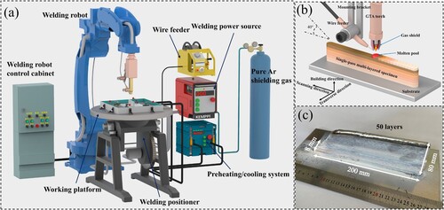
Table 1. Compositions of the feedstock and as-deposited components (wt.%).

Alloys	Al	Zn	Mg	Cu	Fe	Si	Mn
Filler wire	Bal.	8.25	2.09	2.51	0.05	0.03	0.05
As-deposited component	Bal.	7.18	1.92	2.36	0.03	0.01	0.04
Element loss rate	None	12.9%	8.1%	5.9%	40%	66.6%	20%

Figure 2. Heat flux during DSC process of Al-Zn-Mg-Cu components.

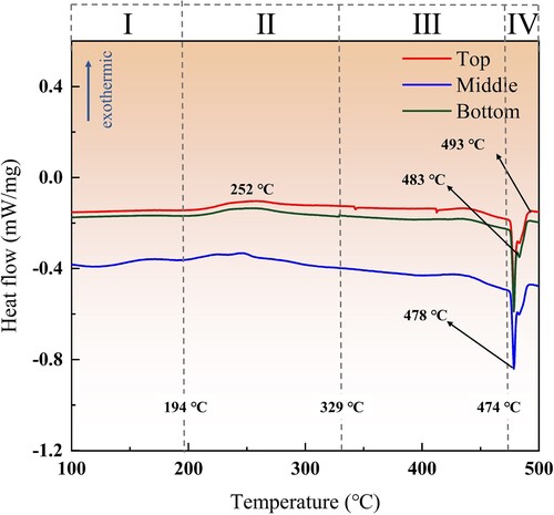
Figure 3. (a) Mechanical property test sampling position, (b) Microstructure observation position, (c) Tensile specimen size, (d) SSRT specimen size (Unit: mm).

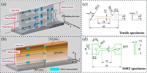
Figure 4. (a) Corrosion solution circulation diagram, (b) SSRT diagram.

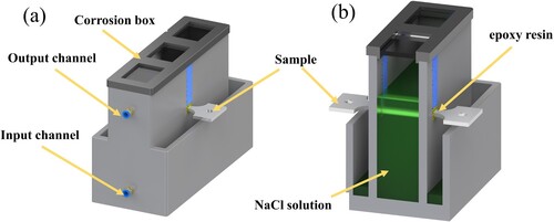
Figure 5. Macroscopic morphology of the deposited structure: (a1) BOT, (a2) Position A in BOT, (a3) Position B in BOT, (b1) BOS, (b2) Position C in BOS, (b3) Position D in BOS.

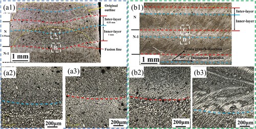
Figure 6. (a1) EBSD orientation diagram of BOT-T, (a2) (001) PF and [001] IPF of BOT-T, (a3) statistical diagram of grain size of BOT-T, (b1) EBSD orientation diagram of BOT-M, (b2) (001) PF and [001] IPF of BOT-M, (b3) statistical diagram of grain size of BOT-M.

Figure 7. (a1) EBSD orientation diagram of BOS-T, (a2) (001) PF and [001] IPF of BOS-T, (a3) statistical diagram of grain size of BOS-T, (b1) EBSD orientation diagram of BOS-M, (b2) (001) PF and [001] IPF of BOS-M, (b3) statistical diagram of grain size of BOS-M.

Figure 8. (a) Low magnification BSE image of BOT-M, (b) High magnification BSE image of BOT-M, (c) Low magnification BSE image of BOS-M, (d) High magnification BSE image of BOS-M, (e) EDS line scan results.

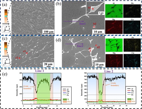
Table 2. Chemical compositions of second phases (at%).

Point	Al	Zn	Mg	Cu	Fe	Si	Mn
b1	62.22	13.82	14.37	9.50	0.05	0.01	0.04
b2	52.88	17.00	18.36	11.60	0.11	0.01	0.08
c1	69.34	10.84	11.92	7.79	0.02	0.01	0.08
c2	48.41	17.91	20.06	13.47	0.08	0.02	0.05
d1	54.71	16.15	17.23	11.76	0.11	0.01	0.08
d2	66.54	11.98	11.26	10.30	0.00	0.01	0.05

Figure 9. XRD patterns of Al-Zn-Mg-Cu alloy as-deposited components.

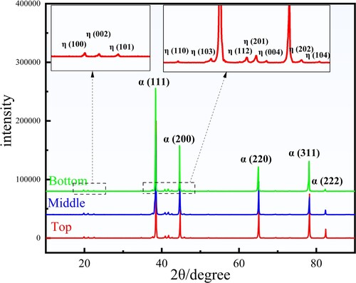
Figure 10. TEM bright field image and SAED pattern of the second phases: (a1) The bright field image of the skeletal second phases at the triangle and (a2) the corresponding SAED pattern, (b1) The bright field image of the strip-shaped second phases and (b2) Corresponding SAED pattern, (c1) Point-like second phases and (c2) corresponding SAED image, (c3) corresponding HAADF-STEM image and (c4) EDS element scanning results.

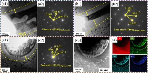
Figure 11. TEM bright field images of precipitated phases at different positions: (a) Top region, (b) Middle region, (c) Bottom region. Respectively, 1 is a low-magnification image containing MPs, 2 is a high-magnification image containing MPs, 3 is a low-magnification image containing GBPs, and 4 is a high-magnification image containing GBPs.

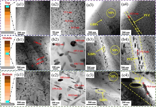
Table 3. Summaries of statistical parameters of MPs, GBPs and PFZ at different locations.

location	MPs size (nm)	GBPs size (nm)	PFZ width (nm)
Top	12.6 ± 3.5	40.2 ± 8.1	29.0 ± 5.7
Middle	274.5 ± 138.6	125.5 ± 27.9	133.4 ± 22.7
Bottom	283.5 ± 75.2	316.7 ± 41.3	523.5 ± 73.9

Figure 12. TEM characterisation of the precipitated phases: (a1) High-resolution image of the Top region obtained along the [110]_Al zone axis, (a2–a4) Corresponding FFT diffractograms obtained from the lattice images of these three different precipitates in a1, (b1) Bright field image of the Middle region, (b2) SAED pattern of b1, (b3) High-resolution image of the polygonal precipitated phases with indexed FFT pattern, (b4) High-resolution image of the rectangular precipitated phases with indexed FFT pattern.

Figure 13. Microhardness distribution on BOT surface.

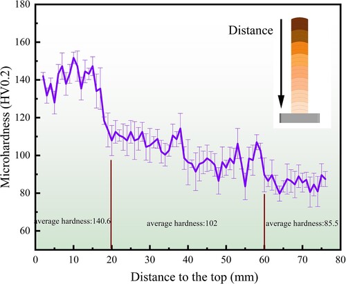
Figure 14. (a) Typical tensile stress-strain curve, (b) strength and elongation.

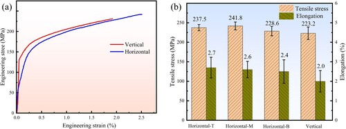
Figure 15. (a1) Typical fracture of horizontal sample, (a2) macroscopic image of fracture section, (a3) secondary electron image of fracture of Inner-layer, (a4) secondary electron image of fracture of Inter-layer. (b1) Typical fracture of vertical sample, (b2) macroscopic image of the fracture section, (b3) high-magnification secondary electron image of the fracture section, (b4) high-magnification backscattered electron image of the fracture section.

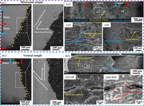
Figure 16. (a) Typical stress-strain curve after SSRT in air, (b) typical stress-strain curve after SSRT in corrosive solution, (c) typical stress-strain curves after SSRT in air and corrosive solution, (d) loss rates of tensile strength and elongation.

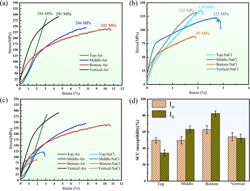
Table 4. SSRT parameters and correlative SCC indexes.

State	Medium	UTS/MPa	Elongation/%	Fracture time/h	Iσ/%	Iδ/%
Top	Air	278.5	3.2	23.8	49.9	34.3
	Solution	139.4	2.1	16.1
Middle	Air	243.2	7.6	54.2	49.8	63.2
	Solution	121.9	2.8	20.4
Bottom	Air	242.3	10.8	70.2	62.8	82.4
	Solution	90.2	1.9	13.3
Vertical	Air	292.2	4.4	32.3	54.1	52.3
	Solution	134.2	2.1	13.4

Figure 17. Fracture morphology after SSRT in air and NaCl solution.

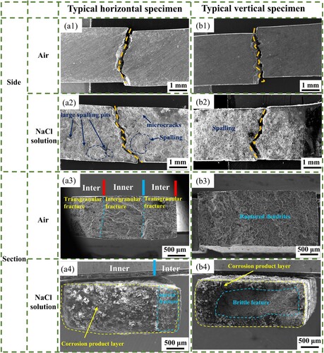
Figure 18. (a) The relationship between R and V, (b) The distribution of temperature gradient and growth rate on the molten pool boundary, (c) The influence of temperature gradient G and growth rate R on the morphology and size of the solidified structure [62].

Figure 19. (a) Schematic diagram of molten pool crystallization, (b) The true morphology of grain orientation of cyclic interlayer structure.

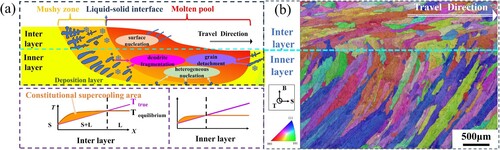
Figure 20. (a) Second phases precipitated by quenching, (b) MPs precipitated by quenching (dark field phases), (c) Dislocation, (d) Schematic diagram of the influence of thermal cycles on the precipitation process.

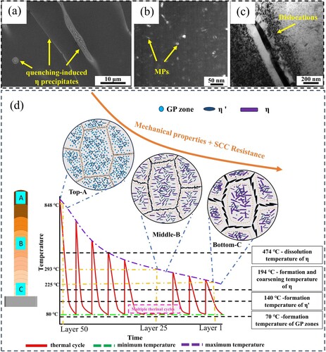
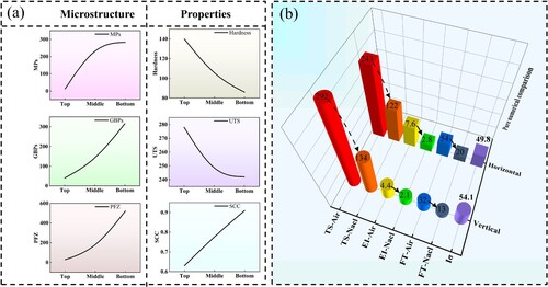
Figure 21. (a) Inhomogeneity of microstructure and mechanical properties, (b) Anisotropy of mechanical properties and SCC susceptibility.

Kou S. Welding metallurgy. Hoboken (NJ): A John Wiley & Sons, Inc.; 2003, 17–20.

 Google Scholar

Data availability statement

The data that support the findings of this study are available from the corresponding author upon reasonable request.