Heat treatment effects and variant selection in multi-material laser powder bed fusion of FeNi- and CoCr-based alloys

Figures & data

Table 1. Chemical composition of maraging steel and CoCrMo feed powders (in wt.%).

Material	Fe	Co	Cr	Ni	Mo	Ti	Mn	Si	C
Maraging	Balance	9.30	–	18.00	4.90	1.10	0.15	0.10	0.03
CoCrMo	0.75	Balance	30.00	0.10	7.00	–	1.00	1.00	0.16

Figure 1. Schematic illustration of three heat treatment schedules (HT1, HT2 and HT3) employed in this work, with the relevant temperatures and holding times considered for both alloys.

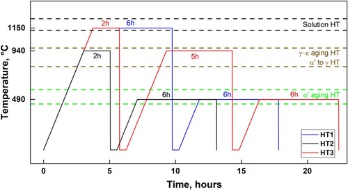
Figure 2. Microstructural features of the as-built MMAM component: (a) transition zone, (b, d) maraging steel cellular structure and (c, e) CoCrMo cellular structure.

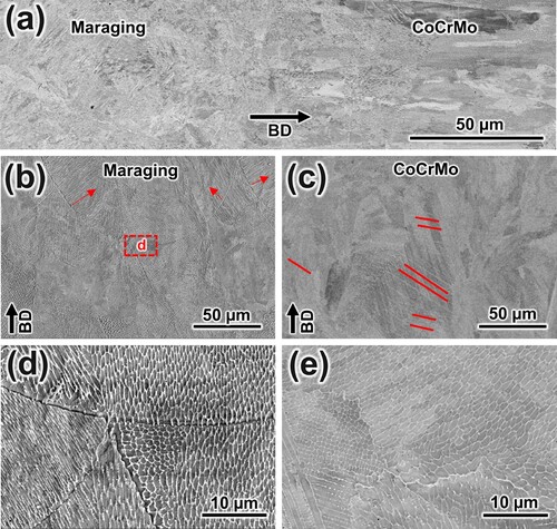
Figure 3. Texture development in the transition zone of the as-built sample: (a) phase map showing fcc and bcc structures, (b) inverse pole figure colour map, (c) kernel average misorientation maps, (d,e,h,i) EDS maps for Co, Cr, Fe and Ni, respectively, (f) corresponding legends for a–c, (g) IPF representation of fcc grains and (j) IPF representation of bcc grains.

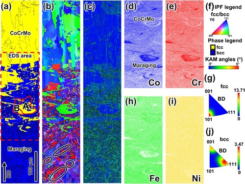
Figure 4. Microstructural features after HT1: (a) transition zone, (b, d) maraging steel lath structure and (c, e) CoCrMo twin structure.

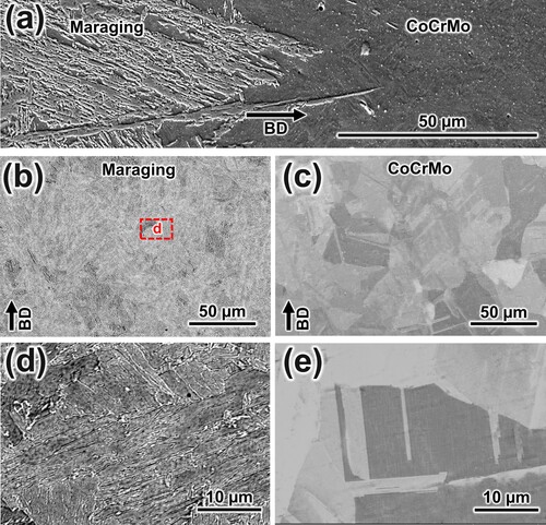
Figure 5. Texture development in the transition zone of the HT1 sample: (a) phase map showing fcc and bcc structures, (b) inverse pole figure colour map, (c) kernel average misorientation maps, (d,e,h,i) EDS maps for Co, Cr, Fe and Ni, respectively, (f) corresponding legends for a–c, (g) IPF representation of fcc grains and (j) IPF representation of bcc grains.

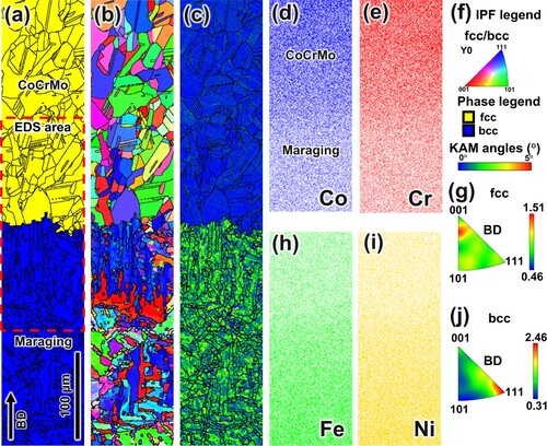
Figure 6. High resolution structures of HT1 sample: (a) TEM-BF images, (b) EDS mapping results and (c) corresponding selected area diffraction pattern.

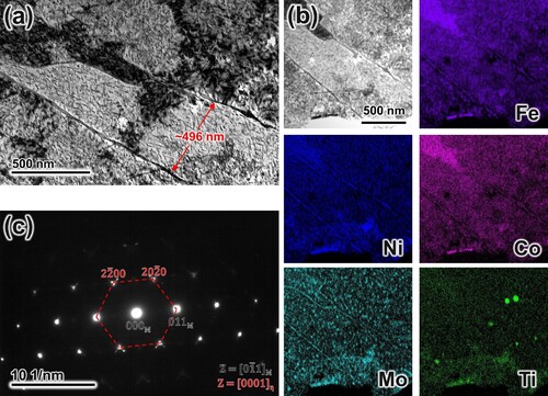
Figure 7. Microstructural features after HT2: (a) transition zone, (b, d) maraging steel lath structure and (c, e) CoCrMo structure.

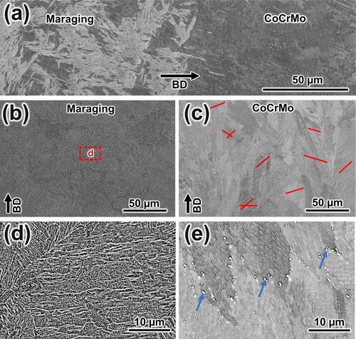
Figure 8. Texture development in the transition zone of the HT2 sample: (a) phase map showing fcc, bcc and hcp structures, (b) inverse pole figure colour map, (c) kernel average misorientation maps, (d,e,h,i) EDS maps for Co, Cr, Fe and Ni, respectively, (f) corresponding legends for a–c, (g) IPF representation of fcc, hcp and bcc grains.

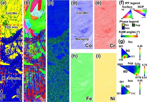
Figure 9. High resolution structures of HT2 sample: (a) TEM-BF images, (b) EDS mapping results and (c) corresponding SAED pattern.

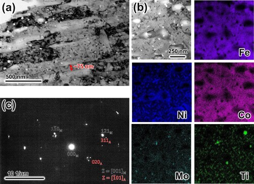
Figure 10. Microstructural features after HT3: (a) transition zone, (b, d) maraging steel lath structure and (c, e) CoCrMo structure.

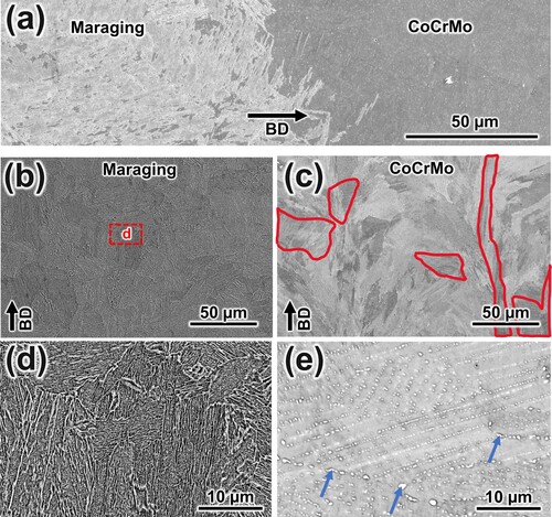
Figure 11. Texture development in the transition zone of the HT3 sample: (a) phase map showing fcc, bcc and hcp structures, (b) inverse pole figure colour map, (c) kernel average misorientation maps, (d,e,h,i) EDS maps for Co, Cr, Fe and Ni, respectively, (f) corresponding legends for a–c, (g) IPF representation of fcc grains, (j) IPF representation of hcp grains and (k) IPF representation of bcc grains.

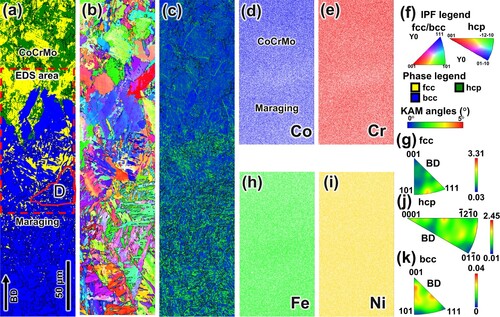
Figure 12. High resolution structures of HT3 sample: (a) TEM-BF images, (b) EDS mapping results and (c) corresponding SAED pattern.

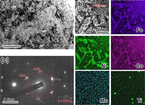
Figure 13. (a) Reconstructed 3D elemental distribution maps combining Ni, Ti and Mo rich precipitates. Statistical proximity histograms for (b) Ni–Ti-based Ni₃Ti precipitates considering the surface value of 4.82 at.% Ti and (c) Mo-based (Fe,Ni,Co)₂(Ti,Mo) considering the surface value of 4.82 at.% Mo.

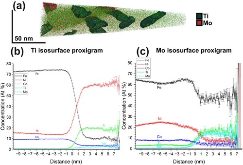
Figure 14. Hardness variation in the transition zones of as-built and heat-treated specimens

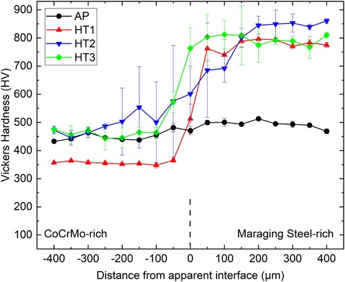
Figure 15. Engineering stress–strain curves from uniaxial tests performed on as-built and heat-treated specimens

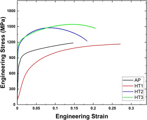
Figure 16. Pole figure analysis of Grain A (a–c) and Grain B (d–f) in as-built samples: (a, d) band contrast with fcc phase IPF colour map (left) and corresponding {100}γ pole figures (right), (b, e) band contrast with bcc phase IPF colour map (left) and corresponding {100}γ pole figures (right), (c, f) band contrast with phase map (left) and comparison of {100}α to the predicted K–S and N–W variants projected along the {111}γ plane.

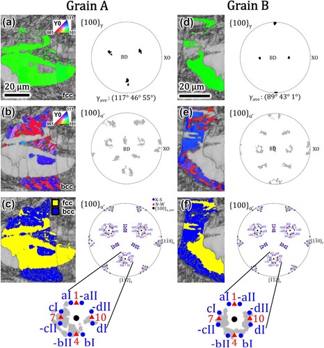
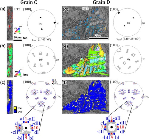
Figure 17. Pole figure analysis of Grain C (a–c) from HT2 and Grain D (d–f) from HT3: (a, d) band contrast with fcc phase IPF colour map (left) and corresponding {100}_γ pole figures (right), (b, e) band contrast with bcc phase IPF colour map (left) and corresponding {100} _α’ pole figures (right), (c, f) band contrast with phase map (left) and comparison of {100}_α’ to the predicted K–S and N–W variants projected along the {111}_γ plane.

Data availability statement

The data that support the findings of this study are available from the corresponding author upon reasonable request.