Design and manufacture of low-frequency acoustic absorption metamaterials with enhanced coupling characteristic

Figures & data

Figure 1. Schematic diagram of MHSTA. (a) Unit structure with related parameters. (b) Various types of unit structures. (c) MHSTA. (d)–(f) Structures of various apertures. (g) Advantageous frequency ranges of units with different n.

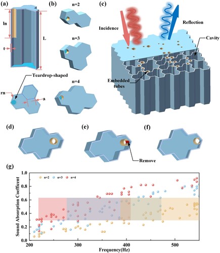
Figure 2. Schematic diagram of the neck section.

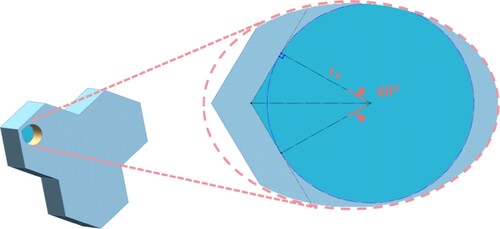
Table 1. Physical parameters and their values.

Physical parameters	Value	Physical parameters	Value
${\rho }_0$	1.21 kg/m^3	$c_0$	343 m/s
$\gamma$	1.4	$\eta$	1.825 × 10^−5 kg/(m·s)
$C_p$	1007 J/(kg·K)	$K$	0.2514 W/(m·K)

Figure 3. Simulation model.

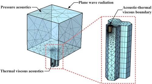
Figure 4. Low-frequency enhancement mechanism of double-unit coupled structure. (a) Sound absorption coefficients with various relative positions of the apertures. (b) Enhancement of absorption peak of various relative positions of the apertures compared with Kirchhoff’s law $({\alpha }_{max1}-{\alpha }_{max2})/{\alpha }_{max2}$. Wherein ${\alpha }_{max1}$ is the absorption peak of various relative positions of the apertures and ${\alpha }_{max2}$ is the absorption peak of Kirchhoff’s law. (c) Acoustic impedances of the structure i and ii. (d) Pressure and velocity of the structure i and ii at 480 Hz.

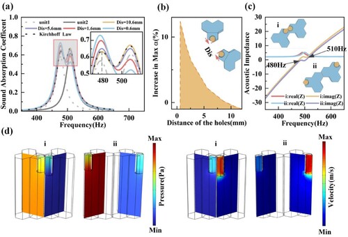
Figure 5. Broadband and uniform enhancement of multi-unit coupling. (a) Comparison of coupling characteristics of coupled 1 and 2. (b) Comparisons of coupling characteristics of coupled 2–4. (c) Four coupling layouts.

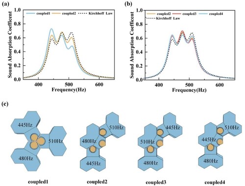
Figure 6. The maximum relative errors and resonance frequency errors between the theories and simulations of single unit. (a) The maximum relative errors. (b) The resonance frequency errors.

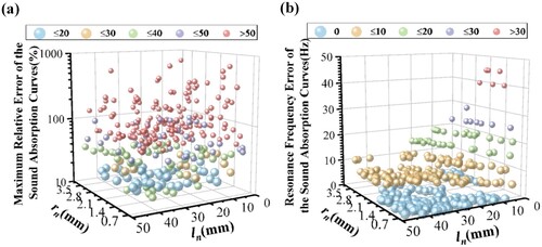
Figure 7. Design strategy of the UIC method for MHSTA.

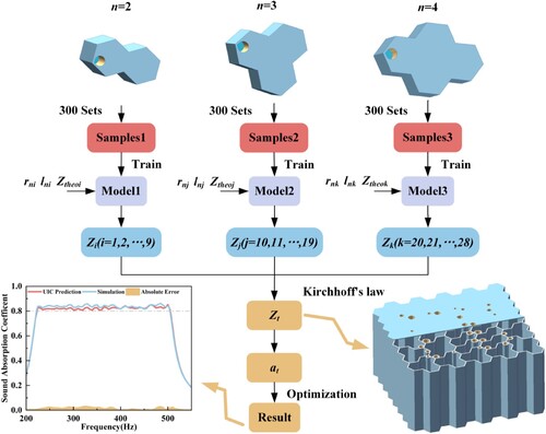
Figure 8. The ANN with various parameters to be trained.

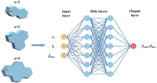
Figure 9. Comparison of acoustic resistances, acoustic reactance and acoustic curves among simulations, theories and UIC methods. (a), (d) and (g) Describe the acoustic resistance. (b), (e) and (h) Describe the reactance. (c), (f) and (i) Describe the acoustic curves.

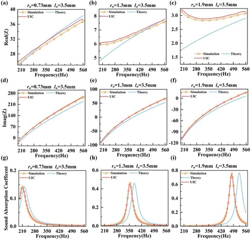
Figure 10. The resonance frequency errors after the UIC method of single unit. (a) The maximum relative errors. (b) The resonance frequency errors.

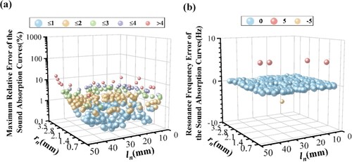
Figure 11. Absorption performance of typical structures in different frequency ranges. (a) Absorption curve, (b) impedance and (c) sound pressure distribution of the cavity in 225–500 Hz. (d) Absorption curve, (e) impedance and (f) sound pressure distribution of the cavity in 230–550 Hz.

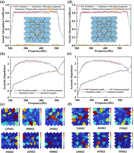
Figure 12. Experimental verification of the performance of acoustic absorption metamaterial in 223–504 Hz. (a) Experimental system. (b) Sample. (c) Comparisons of the UIC, simulation and experiment.

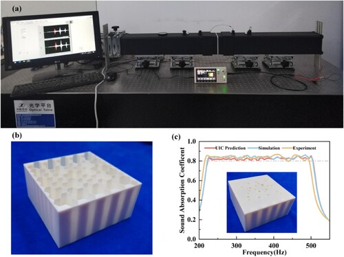
Table 2. Comparison with other advanced metamaterials.

Structure	Absorption performance	Frequency range	Average coefficient	Thickness	Relative bandwidth	extreme difference	Reference
		226–304 Hz	0.93	56 mm ≈ 1/27 λmax	29.4%	≈0.18	[18]
		282–480 Hz	0.98	≈70 mm ≈ 1/17 λmax	52.0%	≈0.10	[19]
		240–500 Hz	≈0.84	50 mm ≈ 1/28 λmax	70.3%	≈0.20	[13]
		280–420 Hz	≈0.91	59 mm ≈ 1/21 λmax	40%	≈0.20	[36]
		200–315 Hz	≈0.92	73 mm≈1/23 λmax	44.7%	≈0.20	[34]
		299–623 Hz	≈0.88	52 mm ≈ 1/22 λmax	70.3%	≈0.26	[20]
		223–504 Hz	0.83	50 mm ≈ 1/31 λmax	77.3%	≈0.05	This work

Table 3. Comparison with other metamaterials optimisation with neural network.

Structure	Network structure	Sample size	Error	Reference
		100000	<0.06 (MAE)	[36]
		20000	0.065 (maximum error)	[35]
		900	0.033 (maximum relative error)	This work

Lue C, Tang S, Wu J-L, et al. Low-frequency acoustic absorption realized by ultrasparse coiling-up metasurfaces. Results Phys. 2023;49:106488. doi:10.1016/j.rinp.2023.106488

 Web of Science ®Google Scholar

Zhang L, Zhang W, Xin F. Broadband low-frequency sound absorption of honeycomb sandwich panels with rough embedded necks. Mech Syst Signal Process. 2023;196:110311. doi:10.1016/j.ymssp.2023.110311

 Web of Science ®Google Scholar

Xu W, Liu J, Yu D, et al. Coherent coupling based meta-structures for high acoustic absorption at 220-500 Hz frequency. Appl Acoust. 2021;182:108181. doi:10.1016/j.apacoust.2021.108181

 Web of Science ®Google Scholar

Wang Z-W, Chen A, Xu Z-X, et al. On-demand inverse design of acoustic metamaterials using probabilistic generation network. Sci China Phys Mech Astron. 2023;66(2):224311. doi:10.1007/s11433-022-1984-1

 Web of Science ®Google Scholar

Mahesh K, Ranjith S, Mini R. A deep autoencoder based approach for the inverse design of an acoustic-absorber. Eng Comput. 2023;40:297–300. doi:10.1007/s00366-023-01789-9.

 Web of Science ®Google Scholar

Li Q, Dong R, Mao D, et al. A compact broadband absorber based on helical metasurfaces. Int J Mech Sci. 2023;254:108425. doi:10.1016/j.ijmecsci.2023.108425

 Web of Science ®Google Scholar

Liu L, Xie L-X, Huang W, et al. Broadband acoustic absorbing metamaterial via deep learning approach. Appl Phys Lett. 2022;120(25):251701. doi:10.1063/5.0097696

 Web of Science ®Google Scholar

Data availability statement

The data that support the findings of this study are available from the corresponding author upon reasonable request.