Figures & data
Figure 1. Clinical history.
Figure 2. The fixtures over time, with the white fixtures and abutments corresponding to the interventions and changed parts. RH, LH: right and left humerus; RR, LR: right and left radial; RU, LU: right and left ulna.
Figure 3. A. A SEM image of the Pt deposit at the site of interest. B. Trenches were cut on both sides of the Pt layer. C. The cut-out lamella was soldered to a TEM grid before final thinning. D. The final thinning was done with decreasing ion beam currents to obtain electron transparency.
Figure 4. A. Micrograph of the apical part of the implant. Trabecular bone is growing into the hollow apex of the implant and is also growing at the implant surface. B. Bone growth into the hollow part of the implant following the implant surface. C. This high-magnification optical micrograph shows the bone-implant contact in the hollow part of the implant.
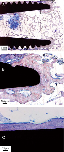
Figure 5. A. Overview of the implant fracture and the closest threads. B. A large amount of bone-implant contact within the threads closest to the implant fracture.
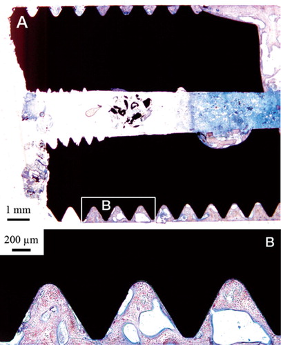
Figure 6. A thread completely filled with mature compact bone.
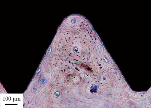
Figure 7. The distribution of bone area within threads (black bars) and bone-implant contact (gray bars) along the implant threads from fracture zone to apex. The axis est threads. B. A large amount of bone-implant contact represents the amount in percentage, within the threads closest to the implant fracture.
Figure 8. TEM bright-field image of the sample. The arrows show the apatite layer (∼200 nm) closest to the implant surface. The arrowheads show a layer with high diffraction contrast, containing HA crystals (∼200 nm). (*Artifact of preparation).
Figure 9. A. An EFTEM image of the sample generated from electrons with zero-loss energy. B. Image generated by electrons with an energy loss characteristic of titanium (Ti). C. Image generated by electrons with an energy loss characteristic of calcium (Ca). D) Image generated by electrons with an energy loss characteristic of carbon (C).
Figure 10. A high-resolution image of the interface zone where crystalline hydroxyapatite (HA) is present at the implant surface according to the bandwidth. There is an amorphous zone between the HA and the titanium, which most likely corresponds to amorphous titanium oxide.