Adjuvant therapies of bone graft around non-cemented experimental orthopedic implants stereological methods and experiments in dogs

Figures & data

Figure 1. Observation time

Figure 2. Non‐coated and HA‐coated plasma spray porous Ti implants with a 2.5 mm gap

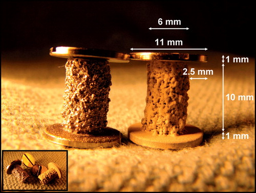
Figure 3. Implant sites

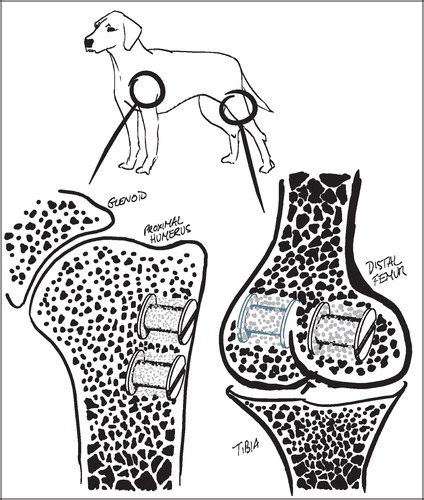
Table 1.  Mechanical specimens' diameter and height

Study		Diameter		Height
		mean	(sd)	mean	(sd)
I	all	5.69	0.24	3.29	0.33
	Ti	5.75	0.25
	HA	5.63	0.22
II	Ti	5.74	0.20	3.24	0.21
III	Ti	5.96	0.18	3.11	0.32

Figure 4. Transverse section for mechanical testing

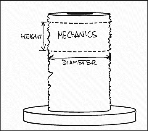
Figure 5. Force‐displacement curve (normalized)

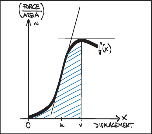
Figure 6. Force‐displacement curve with two peaks

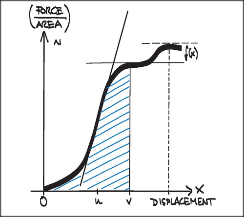
Figure 7. Force and material stress multiplicity at the bone‐implant interface at axial push‐out test

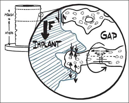
Figure 8. Schematics of cyclic test and push‐out

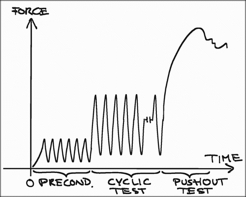
Figure 9. Vertical sectioning technique

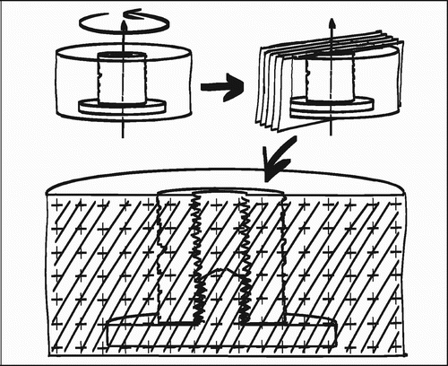
Figure 10. Exhaustive vertical sections (above) and central vertical sections (below)

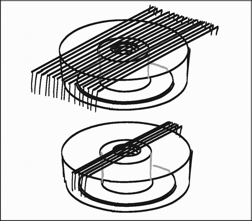
Figure 11. ROI reference line (”approximated surface line”) for placement of Zones 1 and 2

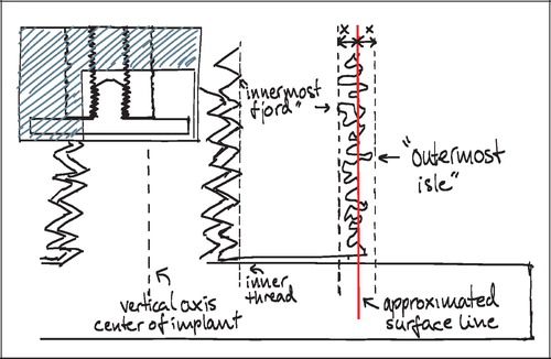
Figure 12. Section offset

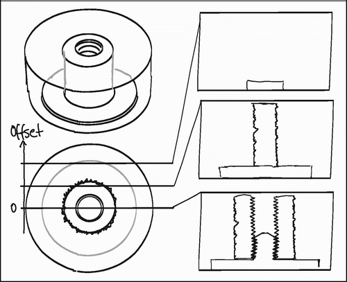
Figure 13. Central section point representation of coaxial volumes

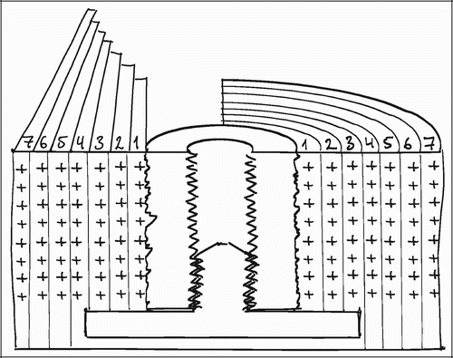
Figure 15. Transverse section of implant (left) and objects with increasing distance to vertical axis

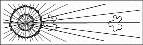
Figure 14. FAVER sections

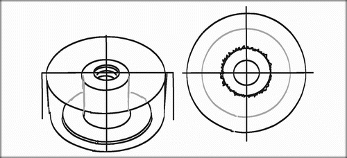
Table 2.  Influence of central section bias on sample tissue volume fraction estimates in Zones B+C+D = Zone 2 (3.5–5 mm). V_VUR: Non‐weighted tissue fraction. V_FAV: distance‐weighted tissue fraction. V/V= V_VUR/ V_FAV

Implant	Bone graft			New bone			Marrow space			Fibrous tissue
	VVUR	VFAV	V/V	VVUR	VFAV	V/V	VVUR	VFAV	V/V	VVUR	VFAV	V/V
1	23.3%	23.1%	1.01	25.9%	26.0%	0.99	50.8%	50.9%	1.00	0.0%	0.0%	‐
2	39.1%	39.6%	0.99	31.3%	31.1%	1.01	29.6%	29.3%	1.01	0.0%	0.0%	‐
3	32.0%	31.8%	1.01	23.8%	24.0%	0.99	44.2%	44.2%	1.00	0.0%	0.0%	‐
4	39.4%	39.2%	1.01	18.4%	18.6%	0.99	42.2%	42.3%	1.00	0.0%	0.0%	‐

Figure 16. Relative tissue representation as a function of distance from the vertical axis, f_T (r)

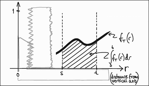
Figure 17. Relative total tissue representation as a function of distance from the vertical axis, f_TOT (r)

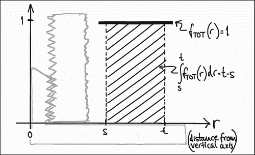
Figure 18. Different geometric centroid for all tissues TOT and a specific tissue T. The area A_TOT, has a gravitational centre in the symmetry line of the ROI; r = ½(t + s). Because of the skew tissue distribution of T, the area A_T, has a gravitational centre to the right of r = ½(t + s.

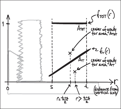
Figure 19. Volume of torus: A×2πr

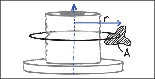
Figure 20. Example of distance‐dependent tissue representation symmetrical around r = ½(t + s)

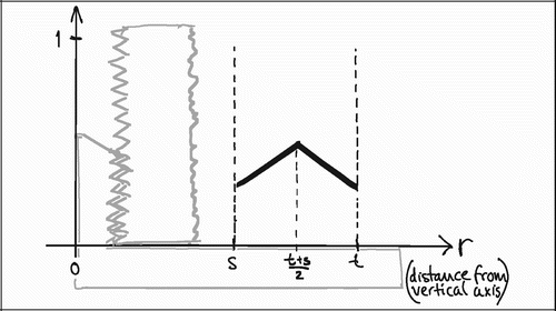
Figure 21. Relative tissue representation as a function of distance from the vertical axis, f_T(r).

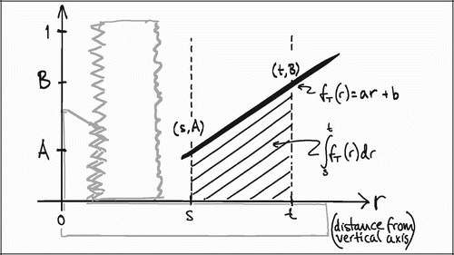
Figure 22. Graphic representation of the V_T(VUR)/V_T(FAVER) ratio in Zone 1 and Zone 2 as a function of A and B (Eq 19 and Eq 20) under the assumptions of linearity and tissue representation throughout the ROI.

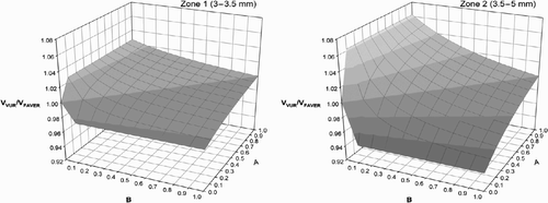
Figure 23. ROI Zones 1 (inner) and 2 (outer)

Figure 24. ROI Zones A, B, C, D and E

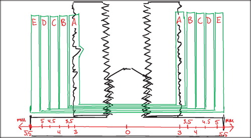
Figure 25. Tissue fractions (not weighted by distance to vertical axis) of the 0.5 mm Zones A‐E of the recount of four implants in study III.

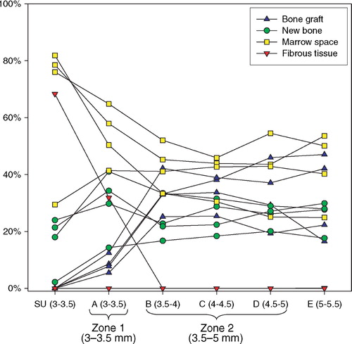
Figure 26. Shadow effect

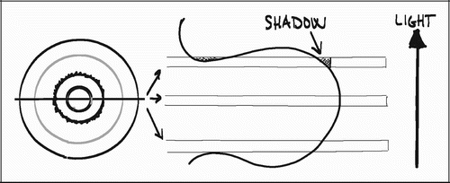
Figure 27. Reducing the amount of sections

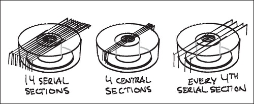
Figure 28. Double counts of four implants

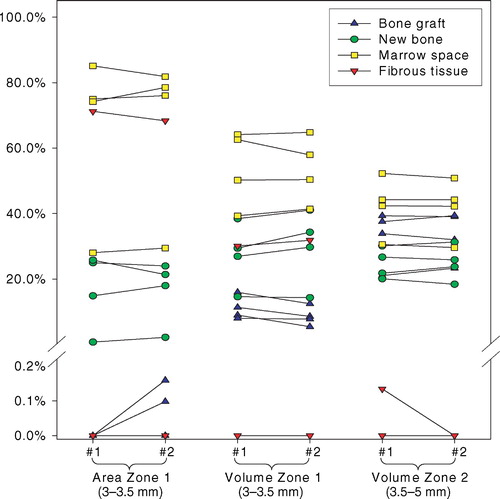
Table 3.  Histomorphometrical reproducibility (CV in percent)

	Bone graft	New bone	Marrow space	Fibrous tissue
Area Zone 1	206	12	3	6
Volume Zone 1	20	8	3	8
Volume Zone 2	4	4	1	283

Figure 29. Overview of studies I‐III

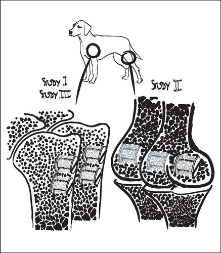
Table 4.  Change relative to control. “0”: no change. “+”: improvement. “−”: deterioration. The double signs “+ +” and “− −” indicate a group best or group worst

	Allograft treatment groups				Implant groups
	Control	BMP	BP	BMP + BP	Ti	HA
Mechanical fixation	0	−	−	− −	0	+
Implant osseointegration	0	0	−	−	0	+
Bone formation	0	+ +	− −	−	0	+
Graft preservation	0	− −	+ +	+	0	0
Fibrous tissue reduction	0	+ +	− −	+	0	+

Figure 30. Study I; representative histology. All four implant sections are from the same dog (Ti implants). Upper left: Control implant with allograft only. Upper right: Allograft added rhBMP‐2. Lower right: Allograft added pamidronate. Lower left: Allograft added rhBMP‐2 and pamidronate in combination.

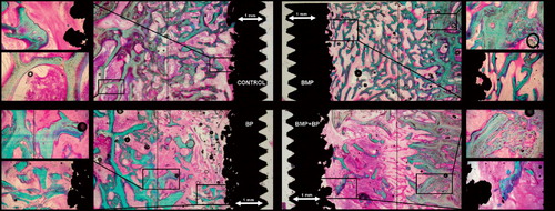
Table 5.  Change relative to control. “0”: no change. “+”: improvement. “−”: deterioration. The double signs “+ +” and “− −” indicate a group best or group worst

	Allograft treatment groups
	Control	Colloss 10 mg	Colloss 20 mg	Colloss 40 mg
Mechanical fixation	0	+	+ +	+
Implant osseointegration	0	+	+ +	+
Bone formation	0	+	+ +	+
Graft preservation	0	−	−	− −
Fibrous tissue reduction	0	+	+	+ +

Table 6.  Change relative to control. “0”: no change. “+”: improvement. “−”: deterioration

	Bone graft treatment groups
	Allograft	Allogr + Colloss E	BGS	BGS + Colloss E
Mechanical fixation	0	0		0
Implant osseointegration	0	0		+
Bone formation	0	0		0
Graft preservation	0	−		+/−
Fibrous tissue reduction	0	0		0

Figure 31. Study III; histology from two implants grafted with β‐TCP granules with Colloss E (left side) and without Colloss E (right side). Implants are not representative of group means and are from different animals.

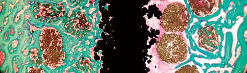
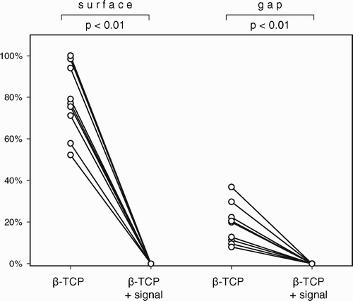
Figure 32. Study III; new bone formation on surface and in gap. Implant pairs interconnected +/− Colloss E (signal).

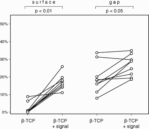
Figure 33. Study III; fibrous tissue on surface and in gap. Implant pairs interconnected +/− Colloss E (signal).