Figures & data
Table 1. Modeled LULC classes, and net change in LULC classes between 1938 and 1992 for the conterminous US. Values represent 1000s km2.
Figure 1. Ecoregions used as the spatial framework for modeling. In the Great Plains and upper Midwest, models were parameterized and run for each Level III ecoregion (27 ecoregions in total). Due to a reduction in resources, models were parameterized and run at the Level II ecoregion scale in the western and eastern US. The base land cover in the figure is the modified 1992 NLCD.
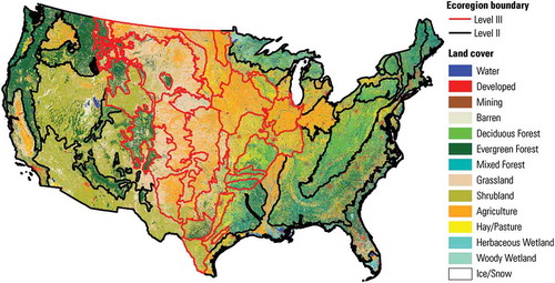
Figure 2. Flowchart depicting Demand construction methodology. Demand construction begins with quantifying the ‘actively modeled’ classes of urban, agriculture (cropland and hay/pasture), wetland, and reservoirs. Quantity (net change) is determined using historical data layers represented in yellow, with USGS Land Cover Trends data used to determine the most likely LULC transitions to achieve net change. The quantity of ‘passively modeled’ classes (primarily natural LULC classes) result from transitions involving the (primarily anthropogenic) actively modeled classes, with USGS Land Cover Trends data used to define transitions between ‘passive’ classes. The final product is a change matrix for each annual model iteration from 1992 back to 1938.
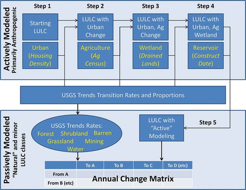
Table 2. Spatially explicit independent variables used in the construction of suitability surfaces.
Figure 3. County-level summary of change from 1938 to 1992 for major aggregate LULC classes.
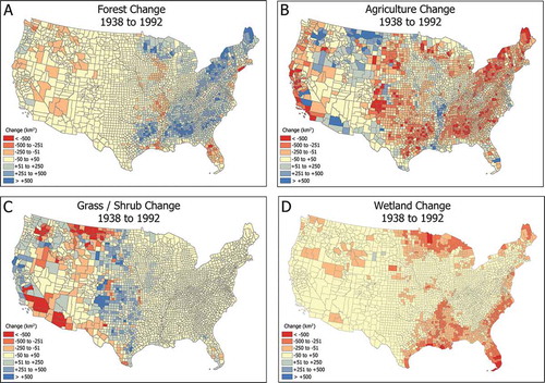
Figure 4. Modeled LULC from 1938 to 1992 for the San Francisco, California area. Major LULC changes noted include 1) areas of urbanization, 2) areas of agricultural loss, and 3) reservoir construction.
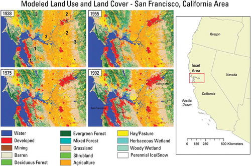
Figure 5. Agreement and disagreement measures between modeled data and USGS Land Cover Trends data for the 84 Level III ecoregions in the conterminous United States. Disagreement is broken down into Quantity Disagreement, and the two elements of Allocation Disagreement (Exchange and Shift).
Figure 6. Total disagreement measures by ecoregion for 1992, and change from 1992 to 1973. Panel A depicts the total disagreement for 1992, representing initial disagreement between the modified 1992 NLCD and the Trends sample blocks. Panel B depicts the percent change in the total disagreement between the modeled and Trends 1973 data.
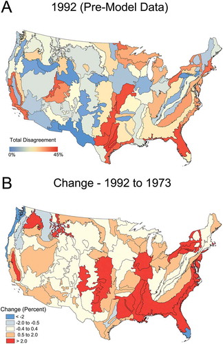
Figure 7. Total area of cropland, hay/pasture, and total agriculture (cropland and hay/pasture) throughout the 1938–1992 simulation period, compared to Agricultural Census data.
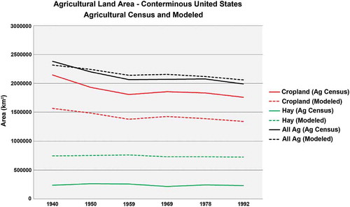
Figure 8. Boxplots of county-level r2 values between modeled LULC and the Agricultural Census data for cropland, hay/pasture, and total agriculture for all counties (national, Panel A), and for Level II (n=15, Panel B) and Level III (n=84, Panel C) ecoregions. Counties were assigned to ecoregions containing the largest areal proportion of that county.
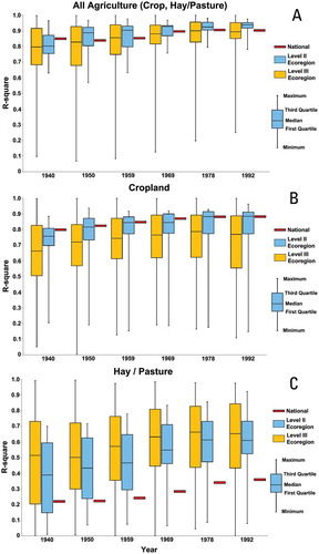
Figure 9. Local Moran’s I of the difference between modeled and Agricultural Census values for the total agriculture, cropland, and hay/pasture, for 1992 and 1938. ‘Cluster of High Values’ represents areas with a statistically significant cluster of overpredicted values (i.e., modeled values higher than Agricultural Census). ‘Cluster of Low Values’ represents areas with a statistically significant cluster of underpredicted values. ‘Outlier – High surrounded by Low’ represents a county with a significantly higher overprediction compared to surrounding counties. ‘Outlier – Low surrounded by High’ represents a count with a significantly lower underprediction compared to surrounding counties.
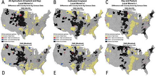
Figure 10. Urban/developed area for the conterminous US as modeled, and for Trends and Housing Density data. Housing density represents areas with > 100 housing units per km2.
Figure 11. ‘Passively’ modeled trends in grassland/shrubland and forest classes, and a comparison with Trends (Sleeter et al. Citation2013), Smith et al. (Citation2004), and Lubowski et al. (Citation2006) data. The modeled and Trends results show combined grassland and shrubland data, while Luboski et al. (2006) depicts a grassland, pasture, and range class. Deciduous, evergreen, and mixed forest classes were combined from these results to compare to the single ‘forest’ class from Trends and Smith et al. (Citation2004).