Uncertainty evaluation approach based on Shannon entropy for upscaled land use/cover maps

Figures & data

Figure 1. Basic scheme of entropy evaluation algorithm for upscaled maps.

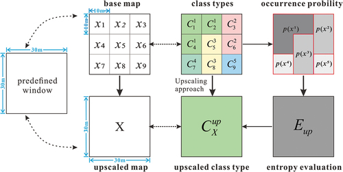
Figure 2. Upscaled maps and their corresponding entropy maps. A subregion was selected to show details of all maps. The upper row shows the land use map at 30 m and its upscaling maps at 150 m, 300 m, 600 m, 900 m, 1500 m, 3000 m, 6000 m, and 9000 m, respectively. The lower row shows the corresponding entropy map as uncertainty evaluation at pixel level for the upscaling map of each row. A subregion was selected to show map details.

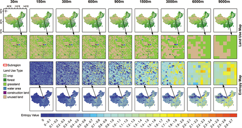
Figure 3. Statistical distribution of the entropy values for each upscaled map. Results in (a), (b), (c), (d), (e), (f), (g), and (h) are calculated from all entropy values of all pixels of each scale (150 m, 300 m, 600 m, 900 m, 1500 m, 3000 m, 6000 m and 9000 m, respectively). Three lines in each sub-figure indicates the quartile positions. The whiskers show 1.5× interquartile range. The red point indicates the mean value of the entropy for each scale.

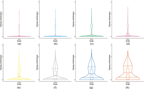
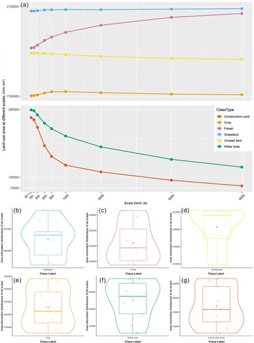
Figure 4. The area of each land use type derived from the upscaled maps, and its statistical distribution for all scales. (a) indicates that the area changes with upscaling for each land use type. (b), (c), (d), (e), (f) and (g) indicate the distribution of the area information of grassland, forest, unused land, crop, water area and construction land, respectively, of all different scales. The centre line indicates the median. The box limits indicate the upper and lower quartiles. The whiskers show 1.5× interquartile range. The centre point indicates the mean value of the data. Each jitter point indicates one data point.