Using microworlds for policymaking in the context of resilient farming systems

Figures & data

Figure 1. The number of cattle farms in the Bourbonnais region [farms] (dashed line – right axis) and the respective average farm size [ha/farm] (solid line – left axis) (source: Agreste FDS_G_0001).

Figure 2. Illustrative behaviour of a stable system after being affected by a disturbance with a limited duration.

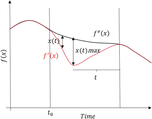
Table 1. Disturbances tested in the model where the disturbance $\sigma$ is defined as per Equation (1)(1) $I=x_{max}=Max\left|f^e\left(x\right)-f{ }^{\mathrm{\prime }}\left(x\right)\right|$(1) as the product of the magnitude of the disturbance (M) and its duration (d) and the angle (θ) between the vector components M and d.

Magnitudes durations	0mm/year	−10mm/year	−50mm/year	−100mm/year	−150mm/year	−200mm/year
1 year	0 mm/ θ: 0°	−10 mm/ θ: −5.7°	−50 mm/ θ: −26°	−100 mm/ θ: −45°	−150 mm/ θ: −56°	−200 mm/ θ: −63°
2 years	0 mm/ θ: 0°	−20 mm/ θ: −2.9°	−100 mm/ θ: −14°	−200 mm/ θ: −27°	−300 mm/ θ: −36°	−400 mm/ θ: −45°
3 years	0 mm/ θ: 0°	−30 mm/ θ: −1.9°	−150 mm/ θ: −9.4°	−300 mm/ θ: −18°	−450 mm/ θ: −26°	−600 mm/ θ: −34°

Note that since M has units of mm/year, the disturbances $\sigma$ have units of mm. The angle θ in Table 1 represents the angle between the vector components M and d. We cannot assume that the system will react in the same way to two vectors that have the same magnitude (e.g., $\sigma$ = −200 mm) if their angles are different (e.g., M = −100 mm/year with d = 2 years and M = −200 mm/year with d = 1 year).

Table 2. A summary of the Eur-Agri-SSPs scenarios used in the analysis to explore future trends for the bovine livestock system in the Bourbonnais region and the variables used in the model to generate each scenario.

SCENARIO	STORYLINE	VARIABLES AFFECTED IN THE MODEL
SCENARIO 1: AGRICULTURE ON SUSTAINABLE PATHS	Social and environmental awareness increase steadily and significantly and are reflected in tightened pro-environmental policies. European domestic demand shifts towards plant-based diets and bio-based materials. International trade decreases because short and transparent agricultural supply chains are preferred. Technology develops with a focus on reducing greenhouse gas emissions	Land available for agriculture: decreases 1% per year from 2020 Market size: decreases 1% per year from 2020 Meat demand per capita: decreases 2% per year from 2020 Farm’s technology: increases 1% per year from 2020
SCENARIO 2: AGRICULTURE ON ESTABLISHED PATHS	European development follows historical patterns resulting in slow but steady social, environmental, and technological progress. Agricultural commodities are mostly traded within Europe even though global market integration advances. Depletion of natural resources increases because of continuous growth of the agriculture and food economy, and pro-environmental regulations and resource-efficient technologies are only developed at a moderate pace.	Land available for agriculture: increases 0.5% per year from 2020 Market size: indexed to population growth in Europe. Meat demand per capita: remains at current levels. Farm’s technology: increases 0.5% per year from 2020
SCENARIO 3: AGRICULTURE ON HIGH-TECH PATHS	European residents share a growing faith in technology, material-intensive lifestyles, and trade liberalisation. Individuals’ affinity for technological innovation also affects increasing global demand for European agricultural products. Increased private investments in technological know-how and the education of employees in the agriculture and food systems boost economic growth, which is largely dependent on fossil energy sources.	Land available for agriculture: increases 0.1% per year from 2020 Market size: increases 3% per year from 2020 Meat demand per capita: remains at current levels. Farm’s technology: increases 2% per year from 2020

Figure 3. A causal loop summarising reinforcing loops included in the model representing bovine livestock farms in Bourbonnais.

Note: Signs (“+” or ‘-‘) at arrowheads indicate the polarity of relationships: a “+” denotes that an increase in the independent variable causes the dependent variable to increase, ceteris paribus (and a decrease causes a decrease). Similarly, ‘-‘ denotes that an increase in the independent variable causes the dependent variable to decrease. The loop identifier, R, indicates a reinforcing feedback mechanism, and B indicates a balancing one (see Sterman, 2002).

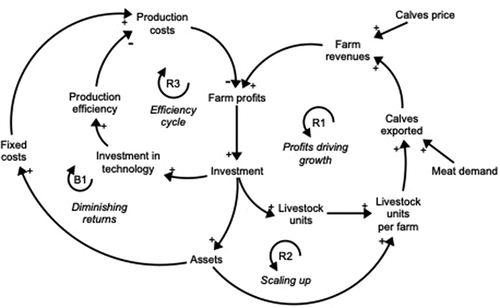
Figure 4. a) A causal loop diagram illustrating the system archetype limits to success and b) an illustrative chart showing the expected relation between farm performance and investment.

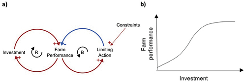
Figure 5. A causal loop summarising some balancing loops included in the model representing bovine livestock farms in Bourbonnais.

Arrows indicate the direction of causality. The plus (+) in the arrowhead indicates a direct relationship between variables, and the minus (-) indicates an inverse relationship between the variables connected. An “R” has been used to denote reinforcing loops and “B” to denote balancing loops.

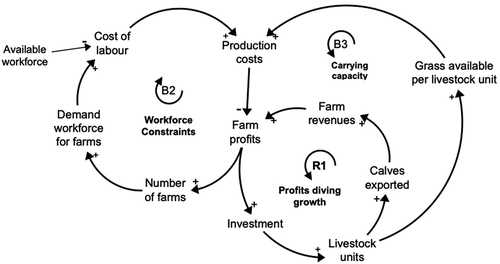
Table 3. Summary of the main inputs and historical data used in the simulation model.

Variable	Use	Source	1999	2000	2001	2002	2003	2004	2005	2006	2007	2008	2009	2010	2011	2012	2013	2014	2015	2016
Utilised Agricultural Area (UAA) [Thousand ha]	Historic data	AGRESTE FDS_SAANR_1	-	503	-	-	-	495	494	490	488	490	488	486	484	484	483	-	-	-
UAA livestock and grassland [Thousand ha]	Historic data	AGRESTE FDS_SAANR_1	-	414	-	-	-	387	387	388	390	389	389	389	388	386	381	-	-	-
%UAA on lease [%]	Model Input	FADN SE030/SE025						77%	78%	78%	78%	77%	77%	77%	76%	77%	78%
Average price per ha (to buy) [Thousand €/ha]	Model Input	AGRESTE terre-net – AGRESTE	2	2	2	2	3	3	3	3	3	4	4	4	4	4	4	4	4	4
Average leasing [Thousand €/ha]	Model input	FADN SE375/SE025						86	92	89	90	91	92	91	92	96	96
Average wage farmer [Thousand €/FTE]	Model input	FADN SE370/SE010	-	-	-	-	-	3	2	2	2	2	2	2	2	2	2	-	-	-
Average farm’s operating cost [Thousand €//LU]	Model input	FADN SE281/SE080	-	-	-	-	-	0.41	0.40	0.39	0.41	0.44	0.47	0.45	0.48	0.55	0.55	-	-	-
Proportion of Assets vs. working capital [unitless]	Model input	FADN SE436/SE510						1.20	1.18	1.19	1.21	1.20	1.18	1.21	1.20	1.20	1.21
Average debt per farm [Thousand €]	Model input	FADN SE485	-	-	-	-	-	143	133	137	147	148	146	153	155	164	181	-	-	-
Average Livestock Units per farm [LU]	Historic data	AGRESTE FDS_SAANR_6, FDS_G_0001						88	92	96	101	106	109	114	114	118	122
Average number of calves per farm [LU]	Historic data	AGRESTE FDS_SAANR_6, FDS_G_0001						18	20	20	22	22	22	23	24	25	25
No. of inhabitants in the region [Thousand people]	Historic data	AGRESTE INSEE	345	345	345	344	344	344	343	343	343	343	342	342	343	341	341	341	340	339
Size of workforce [Thousand FTE]	Historic data	AGRESTE INSEE	-	-	-	-	-	-	-	-	-	-	-	-	199	-	-	-	-	208
No. of inhabitants working in farms (employees and self-employed) [Thousand FTE]	Historic data	AGRESTE FDS_RA_6005_4	-	10	10	10	10	10	10	10	10	10	10	10	-	-	-	-	-	-
Average rainfall precipitation (mm)	Model input	AGRESTE						820	518	723	691	821	640	921	662	817	955	813	580	808
Nb farms (cattle) [Thousand farms]	Historic data	AGRESTE FDS_G_0001	-	4	4	4	4	4	4	3	3	3	3	3	-	-	-	-	-	-

Historical data were used to validate outcomes produced by the model.

Figure 6. A simplified stock-and-flow diagram showing the main structure included in the simulation model representing livestock farming systems in Bourbonnais. Arrows indicate the direction of causality. The plus (+) in the arrowhead indicates a direct relationship between variables, and the minus (-) indicates an inverse relationship between the variables connected. An “R” has been used to denote reinforcing loops and “B” to denote balancing loops. Boxes represent stocks; arrows with valves represent flows. A stock is the accumulation of the difference between its inflows and outflows. Note that the actual model is more complex than this diagram.

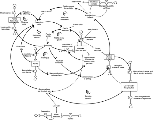
Figure 7. Simulated and historical behaviour for a) average farm size [ha/farm], b) number of farms [farms], c) Jobs in farms [FTE] and d) utilised agriculture area (UAA) [ha] (source for historical behaviour: Agreste FDS_G_0001).

Table 4. Model error for selected variables, where E1 is the error rate and E2 is the error variance.

Variable	E1	E2
UAA dedicated to livestock	0.6%	8.1%
Number farm jobs	0.7%	6.5%
Number livestock farms	1%	7.2%
Number of livestock units per farm	1.2%	10.8%

Figure 8. Simulated behaviour for a) jobs on farms and b) calf exports under the three Eur-Agri-SSPs: Scenario 1 (Sc1): Agriculture on sustainable paths, Scenario 2 (Sc2): Agriculture on established paths, Scenario 3 (Sc3): Agriculture on high-tech paths.

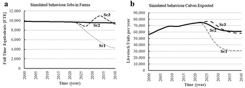
Figure 9. Simulated behaviour for a) jobs on farms and b) calf exports for the disturbances listed in Table 1 under Eur-Agri-SSPs 2 (Agriculture on established paths).

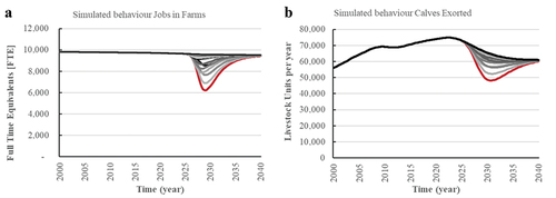
Table 5. Resilience metrics for the disturbances tested in this analysis.

Magnitude [mm/year]	Duration [year]	Impact (I)						Average recovery rates
		Jobs lost [FTE]			Exports lost [LU/year]			Jobs created [FTE/year]			Exports recovered [LU/year^2]
		Scenario 1	Scenario 2	Scenario 3	Scenario 1	Scenario 2	Scenario 3	Scenario 1	Scenario 2	Scenario 3	Scenario 1	Scenario 2	Scenario 3
10	1	25	3	23	59	47	53	12	1	6	54	43	24
50	1	111	11	100	1,469	1,175	661	67	7	34	130	104	59
100	1	217	22	195	2,938	2,350	1,322	82	8	41	573	458	258
150	1	320	32	288	4,407	3,526	1,983	103	10	52	717	574	323
200	1	423	42	381	5,876	4,701	2,644	118	12	59	717	574	323
10	2	99	10	89	116	93	81	44	4	22	111	89	78
50	2	475	48	428	1,155	924	809	116	12	58	222	178	155
100	2	918	92	826	2,888	2,310	3,177	150	15	75	347	382	382
150	2	1,335	134	1,469	5,776	4,621	4,043	100	10	50	556	612	389
200	2	1,727	173	1,900	8,664	6,931	10,397	121	12	61	556	612	667
10	3	219	22	241	168	84	202	69	7	35	54	59	65
50	3	1,028	103	1,131	4,206	2,103	5,047	125	13	63	496	546	595
100	3	1,919	192	2,111	8,411	4,206	10,093	169	17	85	661	727	793
150	3	2,693	269	2,962	12,617	6,309	15,140	218	22	109	740	814	888
200	3	3,645	365	4,010	16,823	8,412	20,188	233	23	117	793	872	952

Table A1. Model equations.

TYPE	VARIABLE	EQUATION	STOCK INITIAL VALUE	UNITS	COMMENT
STOCK	Calves_in_utero[Farm_configuration](t)	Calves_in_utero[Farm_configuration](t – dt) + (Breeding[Farm_ configuration] – Calving_for_Milk[Farm_configuration] – Calving_for_meat_production[Farm_configuration]) * dt	INIT Calves_in_utero[Farm_configuration] = “Initial_Livestock_(LU)”*Livestock_aging_chain_distribution[Calvesinutero]	livestockunit
STOCK	Cows_for_Meat[Farm_configuration](t)	Cows_for_Meat[Farm_configuration](t – dt) + (Calving_for_meat_production[Farm_configuration] + Bought_fattening_cattle[Farm_configuration] – slaughtering_rate[Farm_configuration]) * dt	INIT Cows_for_Meat[Farm_configuration] = (Livestock_aging_chain_distribution[Calves]*”Initial_Livestock_(LU)”+Livestock_aging_chain_distribution[Heifers]*”Initial_Livestock_(LU)”+Livestock_aging_chain_distribution[Mature]*”Initial_Livestock_(LU)”)*(1-Fraction_of_Calves_for_Milk_Production)	livestockunit
STOCK	Mature_Milk_Cows[Farm_configuration](t)	Mature_Milk_Cows[Farm_configuration](t – dt) + (First_Calving[Farm_configuration] – Culling_Milk_Cows[Farm_configuration]) * dt	INIT Mature_Milk_Cows[Farm_configuration] = “Initial_Livestock_(LU)”*Livestock_aging_chain_distribution[Mature]*Fraction_of_Calves_for_Milk_Production	livestockunit
STOCK	Milk_Calves[Farm_configuration](t)	Milk_Calves[Farm_configuration](t – dt) + (Calving_for_Milk[Farm_configuration] – Maturing[Farm_configuration]) * dt	INIT Milk_Calves[Farm_configuration] = “Initial_Livestock_(LU)”*Livestock_aging_chain_distribution[Calves]*Fraction_of_Calves_for_Milk_Production	livestockunit
STOCK	Milk_Heifers[Farm_configuration](t)	Milk_Heifers[Farm_configuration](t – dt) + (Maturing[Farm_configuration] + Bought_Heifers[Farm_configuration] – First_Calving[Farm_configuration]) * dt	INIT Milk_Heifers[Farm_configuration] = “Initial_Livestock_(LU)”*Livestock_aging_chain_distribution[Heifers]*Fraction_of_Calves_for_Milk_Production	livestockunit
FLOW	Bought_fattening_cattle[Farm_configuration]	Change_in_cows_for_meat+slaughtering_rate-Calving_for_meat_production		livestockunit/Years
FLOW	Bought_Heifers[Farm_configuration]	MAX(Heifers_to_increase_milk_LU+Culling_Milk_Cows-Calving_for_Milk, 0)		livestockunit/Years
FLOW	Breeding[Farm_configuration]	Mature_Milk_Cows/Years_between_breeding		livestockunit/Years
FLOW	Calving_for_meat_production[Farm_configuration]	Calves_in_utero/Pregnancy_Time*(1-Fraction_of_Calves_for_Milk_Production)		livestockunit/Years
FLOW	Calving_for_Milk[Farm_configuration]	Calves_in_utero/Pregnancy_Time*Fraction_of_Calves_for_Milk_Production		livestockunit/Years
FLOW	Culling_Milk_Cows[Farm_configuration]	Mature_Milk_Cows/Fattering_time_Milk_Cow		livestockunit/Years
FLOW	First_Calving[Farm_configuration]	Milk_Heifers/Time_between_Calves		livestockunit/Years
FLOW	Maturing[Farm_configuration]	Milk_Calves/Maturing_Time		livestockunit/Years
FLOW	slaughtering_rate[Farm_configuration]	Cows_for_Meat/Fattering_Time		livestockunit/Years
DATA	Average_Fattening_time[Farm_configuration]	2		Years
EQUATION	Average_Weigh_per_cow[Farm_configuration]	Initial_Average_weight_per_LU*Effect_of_fattening_time_on_weight* Effect_of_forage_availability_on_weight		Ton/livestockunit
EQUATION	Average_weight_milk_cow[Farm_configuration]	Initial_Average_weight_per_LU*Effect_of_fattening_time_on_weight_milk_cow* Effect_of_forage_availability_on_weight_milk_cows		Ton/livestockunit
EQUATION	Biomass_Grasslands_available_Livestock[Farm_configuration]	Land.Grassland_Area*Grassland_yield		Ton/years
EQUATION	Change_in_cows_for_meat[Farm_configuration]	(Finance.Desired_LU_meat-Cows_for_Meat)/Time_to_Adjust_Livestock		livestockunit
EQUATION	Desired_Livestock[Farm_configuration]	Land.Area_Livestock*.022		livestockunit
EQUATION	Claves exported	Calves exported per farm × Number of farms		livestockunit/Years
EQUATION	Calves exported per farm	Cows for meat/dt		livestockunit/Years/Farm
TIME SERIES	Effect_of_fattening_time_on_weight[Farm_configuration]	GRAPH(Relative_Fattening_time) Points: (0.000, 0.000), (0.200, 0.242), (0.400, 0.500), (0.600, 0.700), (0.800, 0.900), (1.000, 1.000), (1.200, 1.050), (1.400, 1.100), (1.600, 1.125), (1.800, 1.150), (2.000, 1.150)		Dimensionless
EQUATION	Farm profits	Farm income -Production Cost		Euros/Years
TIME SERIES	Effect_of_fattening_time_on_weight_milk_cow[Farm_configuration]	GRAPH(Relative_Fattening_time_Milk_Cows) Points: (0.000, 0.000), (0.200, 0.242), (0.400, 0.500), (0.600, 0.700), (0.800, 0.900), (1.000, 1.000), (1.200, 1.050), (1.400, 1.100), (1.600, 1.125), (1.800, 1.150), (2.000, 1.150)		Dimensionless
TIME SERIES	Effect_of_forage_availability_on_Milk_production_cost[Farm_configuration]	GRAPH(Percentage_of_forage_requirement_fulfilled) Points: (0.8000, 0.431), (0.8200, 0.600), (0.8400, 0.708), (0.8600, 0.800), (0.8800, 0.869), (0.9000, 0.920), (0.9200, 0.980), (0.9400, 1.000), (0.9600, 1.000), (0.9800, 1.000), (1.0000, 1.000)		Dimensionless
TIME SERIES	Effect_of_forage_availability_on_weight[Farm_configuration]	GRAPH(SMTH3(Percentage_of_forage_requirement_fulfilled, Average_Fattening_time)) Points: (0.8000, 0.431), (0.8200, 0.600), (0.8400, 0.680), (0.8600, 0.750), (0.8800, 0.820), (0.9000, 0.869), (0.9200, 0.900), (0.9400, 0.940), (0.9600, 0.980), (0.9800, 1.000), (1.0000, 1.000)		Dimensionless
STOCK	Assets(t)	Assets (t – dt) + (Acquisition of assets – Depreciation and dwindle) * dt	INIT Assets = Initial_Capital_Stock	Euros
TIME SERIES	Effect_of_forage_availability_on_weight_milk_cows[Farm_configuration]	GRAPH(SMTH3(Percentage_of_forage_requirement_fulfilled, Fattering_time_Milk_Cow)) Points: (0.8000, 0.431), (0.8200, 0.600), (0.8400, 0.680), (0.8600, 0.750), (0.8800, 0.820), (0.9000, 0.869), (0.9200, 0.900), (0.9400, 0.940), (0.9600, 0.980), (0.9800, 1.000), (1.0000, 1.000)		Dimensionless
DATA	“Farm_Size_(LU/UAA)”[Farm_configuration]	0.0216		livestockunit/km2	An average of 52 LU in 88 ha (including 32 ha grassland)
DATA					http://www.filiere-laitiere.fr/en/key-figures/50-facts-about-french-dairy-industry
DATA	Fattering_Time	2		Years
DATA	Fattering_time_Milk_Cow	4		Years	Assumption
DATA					This assumption will need to be validated. The model behaviour is not sensitive to this assumption.
DATA	forage_intake_per_year	14		Ton/ (livestockunit*year)
DATA	Fraction_of_Calves_for_Milk_Production[Farm_configuration]	0.43		Dimensionless	Excel workbook
EQUATION	GAP_in_Livestock[Farm_configuration]	Finance.Desired_LU_Milk-Total_Milk_livestock_held		livestockunit
EQUATION	Grassland_yield[Farm_configuration]	Initial_Grassland_Yield_dry_matter*Soil.Effect_of_Water_on_Yield		Ton/(Km2*year)
EQUATION	Heifers_to_increase_milk_LU[Farm_configuration]	GAP_in_Livestock/Time_to_Adjust_Livestock		livestockunit/Years
TIME SERIES	Historical_Beef_production	GRAPH(TIME) Points: (2005.00, 0.0), (2006.00, 0.0), (2007.00, 0.0), (2008.00, 0.0), (2009.00, 1490.16), (2010.00, 1519.25), (2011.00, 1557.07), (2012.00, 1477.69), (2013.00, 1404.49), (2014.00, 1419.16), (2015.00, 1452.77), (2016.00, 1464.15), (2017.00, 1442.18), (2018.00, 0.0), (2019.00, 0.0), (2020.00, 0.0)		Thousand Ton/Years
DATA	Initial_Average_weight_per_LU	0.75		Ton/livestockunit
DATA	Initial_Grassland_Yield_dry_matter	32		ton/(year*Km2)
EQUATION	“Initial_Livestock_(LU)”[Farm_configuration]	“Farm_Size_(LU/UAA)”*INIT(Land.Area_Livestock)		livestockunit
DATA	Livestock_aging_chain_distribution[Calves]	0.15		Dimensionless
DATA	Livestock_aging_chain_distribution[Heifers]	0.12		Dimensionless
DATA	Livestock_aging_chain_distribution[Mature]	0.73		Dimensionless
DATA	Livestock_aging_chain_distribution[Calvesinutero]	0.075		Dimensionless
DATA	Maturing_Time	1.5		Years
EQUATION	Milk_Demand_for_Calves[Farm_configuration]	Milk_Calves*Milk_demand_per_calve		Ton/years
DATA	Milk_demand_per_calve	0.45		Ton/ (years*livestockunit)
EQUATION	Milk_for_sale[Farm_configuration]	Milk_Production-Milk_Demand_for_Calves		Ton/years
EQUATION	Milk_Production[Farm_configuration]	Mature_Milk_Cows*Milk_Production_per_cow_per_year		Ton/years
DATA	Milk_Production_per_cow_per_year[Farm_configuration]	1.9		Ton/ (years*livestockunit)	A typical cow produces 6800 liters of milk a year
DATA
DATA					http://www.filiere-laitiere.fr/en/key-figures/50-facts-about-french-dairy-industry
EQUATION	Percentage_of_forage_requirement_fulfilled[Farm_configuration]	MIN(Biomass_Grasslands_available_Livestock/Required_Forage, 1)		Dimensionless
DATA	Pregnancy_Time	1		Years
TIME SERIES	Reference_mode_Total_Livestock	GRAPH(TIME) Points: (2005.00, 6,075,040), (2006.00, 6,200,000), (2007.00, 6,295,100), (2008.00, 6,300,000), (2009.00, 6,000,000), (2010.00, 5,557,420), (2011.00, 5,300,000), (2012.00, 5,000,000), (2013.00, 5,035,170), (2014.00, 5,100,000), (2015.00, 5,200,000), (2016.00, 5,460,730), (2017.00, 5,500,000)		livestockunit
TIME SERIES	Reference_model_Milk_for_sale	GRAPH(TIME) Points: (2005.00, 3,496,000), (2006.00, 3,496,000), (2007.00, 3,496,000), (2008.00, 3,496,000), (2009.00, 3,496,000), (2010.00, 3,472,000), (2011.00, 3,383,000), (2012.00, 3,564,000), (2013.00, 3,572,000), (2014.00, 3,391,000), (2015.00, 3,299,000), (2016.00, 3,294,000), (2017.00, 3,230,000)		Ton/years
EQUATION	Relative_Fattening_time[Farm_configuration]	Fattering_Time/Average_Fattening_time		Dimensionless
EQUATION	Relative_Fattening_time_Milk_Cows[Farm_configuration]	Fattering_time_Milk_Cow/Average_Fattening_time		Dimensionless
EQUATION	Required_Forage[Farm_configuration]	Total_Livestock*forage_intake_per_year		Ton/years
EQUATION	Sum_Livestock	SUM(Total_Livestock)		livestockunit
DATA	Time_between_Calves	0.75		Years
DATA	Time_to_Adjust_Livestock	5		Years	Assumption
DATA					This assumption will need to be validated. The model behaviour is not sensitive to this assumption.
EQUATION	Total_Livestock[Farm_configuration]	Total_Milk_livestock_held+Cows_for_Meat+Calves_in_utero		livestockunit
EQUATION	Total_meat_produced[Farm_configuration]	Total_meat_produced_Feeder_Cattle+Total_meat_produced_Milk_Cattle		Ton/years
EQUATION	Total_meat_produced_Feeder_Cattle[Farm_configuration]	slaughtering_rate*Average_Weigh_per_cow		Ton/years
EQUATION	Total_meat_produced_Milk_Cattle[Farm_configuration]	Culling_Milk_Cows*Average_weight_milk_cow		Ton/years
EQUATION	Total_Meat_throughput	SUM(Total_meat_produced)/1000		Ton/years
EQUATION	Total_Milk_for_Sale	SUM(Milk_for_sale)		Ton/years
EQUATION	Total_Milk_livestock_held[Farm_configuration]	Milk_Calves+Milk_Heifers+Mature_Milk_Cows		livestockunit
DATA	Years_between_breeding[Farm_configuration]	4		year
STOCK	“%_UAA_used_for_crops”[Farm_configuration](t)	“%_UAA_used_for_crops”[Farm_configuration](t – dt) + (- Change_in_use_of_land[Farm_configuration]) * dt	INIT “%_UAA_used_for_crops”[Farm_configuration] = 1-Initial_%_of_UAA_used_for_Livestock	Dimensionless
STOCK	“%_UAA_used_for_livestock”[Farm_configuration](t)	“%_UAA_used_for_livestock”[Farm_configuration](t – dt) + (Change_in_use_of_land[Farm_configuration]) * dt	INIT “%_UAA_used_for_livestock”[Farm_configuration] = Initial_%_of_UAA_used_for_Livestock	Dimensionless
STOCK	Desired_Km2_UAA[Farm_configuration](t)	Desired_Km2_UAA[Farm_configuration](t – dt) + (Change_on_Desired_UAA[Farm_configuration]) * dt	INIT Desired_Km2_UAA[Farm_configuration] = INIT(Finance.Desire_to_convert_arable_land)	km2
STOCK	No_Utilised_Agricultural_Area(t)	No_Utilised_Agricultural_Area(t – dt) + (- Change_of_agricultural_area[1] – Change_of_agricultural_area[2] – Change_of_agricultural_area[3] – Change_of_agricultural_area[4] – Change_of_agricultural_area[5]) * dt	INIT No_Utilised_Agricultural_Area  = .06*SUM(Initial_Utilised_Agricultural_Area)	km2
STOCK	“Utilised_Agricultural_Area_(UAA)”[Farm_configuration](t)	“Utilised_Agricultural_Area_(UAA)”[Farm_configuration](t – dt) + (Change_of_agricultural_area[Farm_configuration]) * dt	INIT “Utilised_Agricultural_Area_(UAA)”[Farm_configuration] = Initial_Utilised_Agricultural_Area	km2
EQUATION	Change_in_use_of_land[Farm_configuration]	GAP_%_UAA_for_Livestock/Time_to_adjust_farming_activity		person/(person*year)
EQUATION	Change_of_agricultural_area[Farm_configuration]	MIN(No_Utilised_Agricultural_Area/DT, Arable_Land_Gap)		km2/years
EQUATION	Change_on_Desired_UAA[Farm_configuration]	(Finance.Desire_to_convert_arable_land-Desired_Km2_UAA)/Time_to_adjust_Perception		km2/years
EQUATION	Arable_Land_Gap[Farm_configuration]	(Desired_Km2_UAA-”Utilised_Agricultural_Area_(UAA)”)/Time_to_Adjust_Demand		km2/years
EQUATION	Area_for_Crops_and_Grain[Farm_configuration]	MAX(“%_UAA_used_for_crops”*”Utilised_Agricultural_Area_(UAA)”, 0)		km2
EQUATION	“Area_for_livestock_(including_Grasslands)”[Farm_configuration]	“Utilised_Agricultural_Area_(UAA)”*MIN(“%_UAA_used_for_livestock”, 1)		km2
EQUATION	Area_Livestock[Farm_configuration]	Relation_area_livestock_vs_area_Grassland*”Area_for_livestock_(including_Grasslands)”		km2
EQUATION	GAP_%_UAA_for_Livestock[Farm_configuration]	Finance.Desired_Area_for_Livestock_and_grassland*Finance.Effect_of_crops_gross_margin_on_development_of_Livestock/”Utilised_Agricultural_Area_(UAA)”-”%_UAA_used_for_livestock”		Dimensionless
EQUATION	Grassland_Area[Farm_configuration]	“Area_for_livestock_(including_Grasslands)”*Relation_area_livestock_vs_area_Grassland		km2
DATA	Initial_%_of_UAA_used_for_Livestock[Farm_configuration]	0.63		Dimensionless
DATA	Initial_Utilised_Agricultural_Area[Farm_configuration]	171,510,400		km2
TIME SERIES	Reference_mode_Area_Livestock	GRAPH(TIME) Points: (2005.00, 562,962,000), (2006.00, 550,000,000), (2007.00, 576,405,000), (2008.00, 560,000,000), (2009.00, 550,000,000), (2010.00, 500,319,000), (2011.00, 500,000,000), (2012.00, 490,000,000), (2013.00, 465,470,000), (2014.00, 450,000,000), (2015.00, 480,000,000), (2016.00, 505,428,000), (2017.00, 530,000,000)		km2
TIME SERIES	Reference_mode_Total_UAA	GRAPH(TIME) Points: (2005.00, 860,514,000), (2006.00, 8.6e+08), (2007.00, 876,684,000), (2008.00, 8.5e+08), (2009.00, 8.4e+08), (2010.00, 822,479,000), (2011.00, 8e+08), (2012.00, 7.7e+08), (2013.00, 764,036,000), (2014.00, 7.8e+08), (2015.00, 8.1e+08), (2016.00, 821,257,000), (2017.00, 8.1e+08)		km2
DATA	Relation_area_livestock_vs_area_Grassland[1]	0.5		Dimensionless
DATA	Relation_area_livestock_vs_area_Grassland[2]	0.5		Dimensionless
DATA	Relation_area_livestock_vs_area_Grassland[3]	0.5		Dimensionless
DATA	Relation_area_livestock_vs_area_Grassland[4]	0.5		Dimensionless
DATA	Relation_area_livestock_vs_area_Grassland[5]	0.5		Dimensionless
DATA	Time_to_Adjust_Demand	3		year
DATA	Time_to_adjust_farming_activity	10		year
DATA	Time_to_adjust_Perception	1		Years
EQUATION	Total_Area_Livestock	SUM(“Area_for_livestock_(including_Grasslands)”)		km2
EQUATION	Total_UAA	SUM(“Utilised_Agricultural_Area_(UAA)”)		km2
STOCK	Soil_Organic_Carbon[Farm_configuration](t)	Soil_Organic_Carbon[Farm_configuration](t – dt) + (Soil_Organic_Carbon_Input[Farm_configuration] – Organic_Carbon_Mineralisation_rate[Farm_configuration]) * dt	INIT Soil_Organic_Carbon[Farm_configuration] = 12.5	Ton/(Km2)
STOCK	Soil_Organic_Nitrogen[Farm_configuration](t)	Soil_Organic_Nitrogen[Farm_configuration](t – dt) + (Soil_Organic_Nitrogen_Input[Farm_configuration] – Soil_Organic_Nitrogen_Mineralisation_Rate[Farm_configuration]) * dt	INIT Soil_Organic_Nitrogen[Farm_configuration] = 2.6	Ton/(Km2)
FLOW	Organic_Carbon_Mineralisation_rate[Farm_configuration]	Soil_Organic_Carbon/Average_Carbon_Mineralisation_Time		Ton/(Km2*year)
FLOW	Soil_Organic_Carbon_Input[Farm_configuration]	Organic_Matter_from_Livestock_Manure*Carbon_Share_in_Dry_Matter		Ton/(Km2*year)
FLOW	Soil_Organic_Nitrogen_Input[Farm_configuration]	Organic_Nitrogen_from_livestock_manure		Ton/(Km2*year)
FLOW	Soil_Organic_Nitrogen_Mineralisation_Rate[Farm_configuration]	Soil_Organic_Nitrogen/Nitrogen_Mineralisation_Time		Ton/(Km2*year)
DATA	Add_climate_change_effect	0		Dimensionless
DATA	Average_Carbon_Mineralisation_Time	35		Years
DATA	Carbon_Share_in_Dry_Matter	0.1		Dimensionless
DATA	Effect_of_climate_change	1		Dimensionless
EQUATION	Effect_of_Nitrogen_on_yield[Farm_configuration]	MIN((Nitrogen_Plant_Uptake/Standard_N_required)^Yield_sensitivity_to_Nitrogen, Max_effect_of_Nitrogen_on_Yield)		Dimensionless
DATA	Effect_of_OM_in_Nitrogen_Uptake	0.25		Dimensionless
DATA	Effect_of_OM_in_Water_uptake	0.25		Dimensionless
EQUATION	Effect_of_Water_on_Yield[Farm_configuration]	MIN((Water_Plant_Uptake*Land.Area_for_Crops_and_Grain/Standard_Water_Required)^Yield_sensitivity_to_Water, Max_effect_of_Water_on_Yield)		Dimensionless
DATA	Initial_Plant_Nitrogen_uptake	0.5		Dimensionless
DATA	Initial_Plant_Water_Uptake	0.5		Dimensionless
EQUATION	Initial_Soil_Organic_Matter[Farm_configuration]	INIT(Soil_Organic_Matter)		Ton/(Km2)
DATA	Max_effect_of_Nitrogen_on_Yield	1		Dimensionless
DATA	Max_effect_of_Water_on_Yield	1		Dimensionless
DATA	Nitrogen_content_of_livestock_manure	0.2		Dimensionless
EQUATION	Nitrogen_Mineral[Farm_configuration]	Soil_Organic_Nitrogen_Mineralisation_Rate+Tons_Chemical_Fertilisers_used		Ton/(Km2*year)
DATA	Nitrogen_Mineralisation_Time	35		year
EQUATION	Nitrogen_Plant_Uptake[Farm_configuration]	Nitrogen_Mineral*Plant_uptake_share_of_Nitrogen_Min		Ton/(Km2*year)
EQUATION	Organic_Matter_from_Livestock_Manure[Farm_configuration]	Livestock.Total_Livestock*Tons_Manure_per_LU/(Land.Area_for_Crops_and_Grain+Land.Grassland_Area)		Ton/(Km2*year)
EQUATION	Organic_Nitrogen_from_livestock_manure[Farm_configuration]	Nitrogen_content_of_livestock_manure*Organic_Matter_from_Livestock_Manure		Ton/(Km2*year)
EQUATION	Oscilations	SINWAVE(MAX(Effect_of_climate_change-1, 1), 10/Effect_of_climate_change)		Dimensionless
EQUATION	Percentage_of_Area_held_each_FS[Farm_configuration]	Land.Initial_Utilised_Agricultural_Area/SUM(Land.Initial_Utilised_Agricultural_Area)		Dimensionless
EQUATION	Plant_uptake_share_of_Nitrogen_Min[Farm_configuration]	Initial_Plant_Nitrogen_uptake*Relative_Organic_Matter^Effect_of_OM_in_Nitrogen_Uptake		Dimensionless
EQUATION	Plant_uptake_share_water[Farm_configuration]	Initial_Plant_Water_Uptake*Relative_Organic_Matter^Effect_of_OM_in_Water_uptake		Dimensionless
EQUATION	Rainfall_Precipitation	619*(1+ STEP(Oscilations, 2018)*Add_climate_change_effect)-STEP(250, 2008)+STEP(500, 2010)-STEP(250, 2018)		mm/year
EQUATION	Relative_Organic_Matter[Farm_configuration]	Soil_Organic_Matter/Initial_Soil_Organic_Matter		Dimensionless
EQUATION	Soil_Organic_Matter[Farm_configuration]	Soil_Organic_Carbon*Carbon_Share_in_Dry_Matter		Ton/(Km2)
DATA	Standard_N_required	6		Ton/(Km2*year)
EQUATION	Standard_Water_Required[Farm_configuration]	Water_Required_per_Km2_grassland*Land.Grassland_Area+Water_Required_per_Km2_crop_arable_land*Land.Area_for_Crops_and_Grain		Ton/(Km2*year)
DATA	Tons_Chemical_Fertilisers_used[1]	0.25		Ton/(Km2*year)
DATA	Tons_Chemical_Fertilisers_used[2]	0.25		Ton/(Km2*year)
DATA	Tons_Chemical_Fertilisers_used[3]	0.25		Ton/(Km2*year)
DATA	Tons_Chemical_Fertilisers_used[4]	0.25		Ton/(Km2*year)
DATA	Tons_Chemical_Fertilisers_used[5]	0.25		Ton/(Km2*year)
DATA	Tons_Manure_per_LU	0.025		ton/(livestockunit*year)
EQUATION	Total_Cost_Fertilisers[Farm_configuration]	Market.Fertilisers_Price*Total_Demand_Fertilisers		Euros/Years
EQUATION	Total_Demand_Fertilisers[Farm_configuration]	Tons_Chemical_Fertilisers_used*(Land.Area_for_Crops_and_Grain+Land.Grassland_Area)		Ton/years
EQUATION	Water_Plant_Uptake[Farm_configuration]	MAX(Rainfall_Precipitation*Plant_uptake_share_water, 0)		mm/year
DATA	Water_Required_per_Km2_crop_arable_land	325		mm
DATA	Water_Required_per_Km2_grassland	250		mm
DATA	Yield_sensitivity_to_Nitrogen	0		Dimensionless
DATA	Yield_sensitivity_to_Water	0.25		Dimensionless
STOCK	Account_payable[Farm_configuration](t)	Account_payable[Farm_configuration](t – dt) + (No_Cash_Expenses[Farm_configuration] – Payments_to_suppliers[Farm_configuration]) * dt	INIT Account_payable[Farm_configuration] = 0.9*10^9	Euros
STOCK	Account_Receivable[Farm_configuration](t)	Account_Receivable[Farm_configuration](t – dt) + (Net_Sales[Farm_configuration] – Cash_receipts[Farm_configuration]) * dt	INIT Account_Receivable[Farm_configuration]  = INIT(Total_Revenues_Farming)*2/12	Euros
STOCK	Assets[Farm_configuration](t)	Assets[Farm_configuration](t – dt) + (PP&E_Purchase[Farm_configuration] – Depreciation[Farm_configuration]) * dt	INIT Assets[Farm_configuration] = 2*Initial_Capital_Stock	Euros
STOCK	Capital_Stock[Farm_configuration](t)	Capital_Stock[Farm_configuration](t – dt) + (Increase_Stakeholders_Equity[Farm_configuration]) * dt	INIT Capital_Stock[Farm_configuration] = Initial_Capital_Stock	Euros
STOCK	Cash[Farm_configuration](t)	Cash[Farm_configuration](t – dt) + (Cash_receipts[Farm_configuration] + Debt_acquired[Farm_configuration] + Equity_investment[Farm_configuration] – Cash_disbursements[Farm_configuration] – PP&E_Purchase[Farm_configuration] – Debt_Paid[Farm_configuration] – Dividends_paid[Farm_configuration]) * dt	INIT Cash[Farm_configuration] = 1.8*10^9	Euros
STOCK	Farmers_Debt[Farm_configuration](t)	Farmers_Debt[Farm_configuration](t – dt) + (Debt_increase[Farm_configuration] – Debt_reduction[Farm_configuration]) * dt	INIT Farmers_Debt[Farm_configuration]  = INIT(Cash)-Initial_Capital_Stock	Euros
STOCK	Retained_earnings[Farm_configuration](t)	Retained_earnings[Farm_configuration](t – dt) + (Total_Revenues[Farm_configuration] – Production_cost[Farm_configuration] – Income_tax_payable[Farm_configuration] – Dividends[Farm_configuration] – Operating_Expenses[Farm_configuration] – Interest_paid[Farm_configuration]) * dt	INIT Retained_earnings[Farm_configuration] = 800,000,000	Euros
FLOW	Cash_disbursements[Farm_configuration]	Payments_to_suppliers+Operating_Expenses+Income_tax_payable+Interest_paid		Euros/Years
FLOW	Cash_receipts[Farm_configuration]	Account_Receivable/(Average_credit_given*Convertion_days_to_years)		Euros/Years
FLOW	Debt_acquired[Farm_configuration]	Cash_required*Fraction_of_cash_cover_with_debt		Euros/Years
FLOW	Debt_increase[Farm_configuration]	Debt_acquired		Euros/Years
FLOW	Debt_Paid[Farm_configuration]	Debt_reduction		Euros/Years
FLOW	Debt_reduction[Farm_configuration]	Farmers_Debt/Average_debt_time		Euros/Years
FLOW	Depreciation[Farm_configuration]	Assets/Depreciation_time		Euros/Years
FLOW	Dividends[Farm_configuration]	Annual_return_paid*Retained_earnings/DT		Euros/Years
FLOW	Dividends_paid[Farm_configuration]	Dividends		Euros/Years
FLOW	Equity_investment[Farm_configuration]	Cash_required*(1-Fraction_of_cash_cover_with_debt)		Euros/Years
FLOW	Income_tax_payable[Farm_configuration]	MAX(EBITDA-Interest_paid, 0)*Farm_Tax		Euros/Years
FLOW	Increase_Stakeholders_Equity[Farm_configuration]	Equity_investment		Euros/Years
FLOW	Interest_paid[Farm_configuration]	Debt_interest_rate*Farmers_Debt		Euros/Years
FLOW	Net_Sales[Farm_configuration]	Total_Revenues_Farming		Euros/Years
FLOW	No_Cash_Expenses[Farm_configuration]	Production_Costs_Farming		Euros/Years
FLOW	Operating_Expenses[Farm_configuration]	Workforce.Farming_system_workforce_cost		Euros/Years
FLOW	Payments_to_suppliers[Farm_configuration]	Account_payable/(Average_Credit_time*Convertion_days_to_years)		Euros/Years
FLOW	PP&E_Purchase[Farm_configuration]	Assets_replacement		Euros/Years
FLOW	Production_cost[Farm_configuration]	Production_Costs_Farming		Euros/Years
FLOW	Total_Revenues[Farm_configuration]	Total_Revenues_Farming		Euros/Years
EQUATION	Acid_ratio[Farm_configuration]	(Account_Receivable+Average_Cash)/(Account_payable+Farmers_Debt)		Dimensionless
EQUATION	Annual_Retained_earnings[Farm_configuration]	MEAN(Retained_earnings)		Euros
DATA	Annual_return_paid[Farm_configuration]	0.08		Dimensionless

Sterman, J. (2002). System Dynamics: Systems thinking and modeling for a complex world. Massachusetts Institute of Technology. Engineering Systems Division

 Google Scholar