Figures & data
Figure 1. Part of Manhattan and the city of Timișoara, Romania, shown using Google Maps. Three regions in Timișoara are highlighted where roads have different orientations
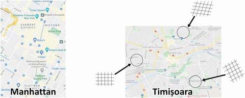
Figure 2. On the left, representative locations within a region (black dots) with three example travel paths and their distances. On the right, the three respective multipliers are shown. Links exist between all possible location pairs, we only show few to avoid congestion
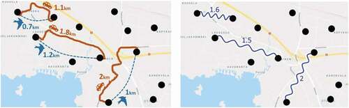
Figure 3. Components used when estimating the distance from source to destination. In our application, the source is a patient’s home and destination is the hospital where the patient needs to visit. The bird-distance between the two is 1.1 km. The two nearest nodes of the overhead graph are connected by a link with T = 1.5
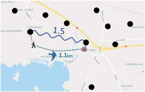
Figure 4. Patient locations and the current health centres in North Karelia (left) and Joensuu city centre (right). The patient locations are shown using a heat-map to preserve anonymity
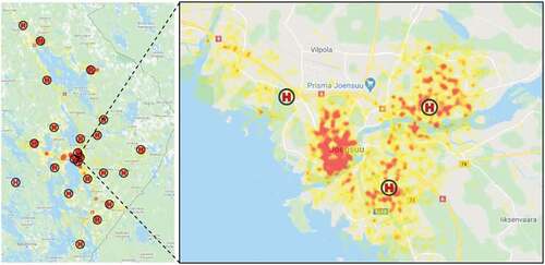
Figure 5. Overhead graphs with 16 nodes generated in the North Karelian region using four different methods. The worst estimation is given by the uniform method. The values in the bottom-right corners are the average approximation errors
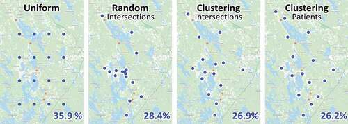
Figure 6. Patient locations clustered with Random Swap algorithm using 16, 32 and 64 clusters; the blue centroids are the nodes of the overhead graph. Selected links from the overhead graph are shown. The links are coloured so that the higher the overhead, the redder the link. The values in the bottom-right corners are the average approximation errors
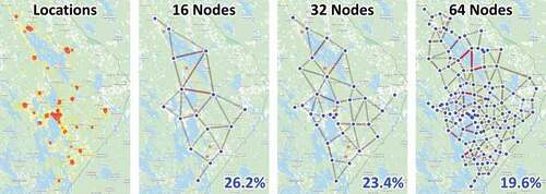
Table 1. The size required by the overhead graph with different number of nodes
Figure 7. Error of the travel-distance estimation using multiple methods. The error of the proposed method is shown when varying the number of nodes of the overhead graph (blue)
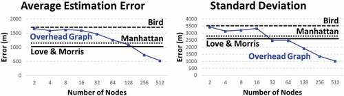
Figure 8. Relative error of the total travel-distance from patients to their nearest health centre. The error of the proposed method is shown when varying the number of nodes of the overhead graph (blue)
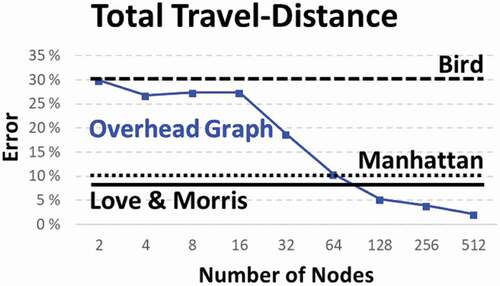
Figure 9. Processing times for all methods. The number of nodes have almost no effect on the speed of the proposed method (blue)
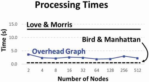
Figure 10. Four examples of A and B locations in the city centre and the bird and road-network distances (top). Estimations are calculated with different node configurations (bottom). The travel-distance is estimated from A to B
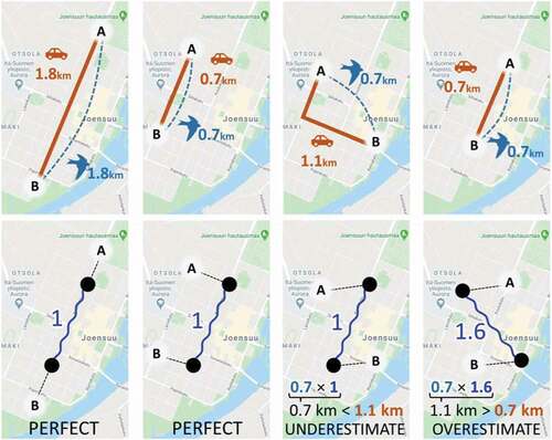
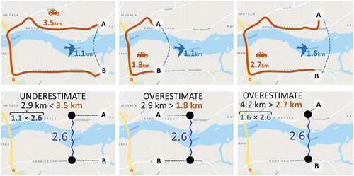
Figure 11. Three examples of A and B locations on opposite sides of the river and the bird and road-network distances (top). Estimations are calculated using the same overhead in all cases. The travel-distance is estimated from A to B