What is a characteristic value for soils?

Figures & data

Figure 1. Results of standard penetration tests in London and Lambeth clays, with engineers’ interpretation of the characteristic value (Bond and Harris 2008).

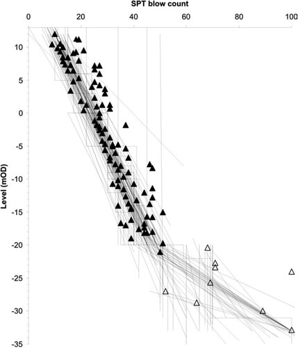
Figure 2. Outcome of equations (1) to (4) for COV = 10% (left) and 30% (right) with respect to number of samples. The multiplier on the mean is the factor $X_k/X_{mean}$, and the partial factor on mean is the inverse.

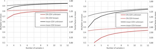
Figure 3. Outcome of equations (1) to (4) for n = 4 and 10 with respect to COV. The multiplier on the mean is the factor $x_k/\mu \left(x\right)$, and the partial factor on mean is the inverse.

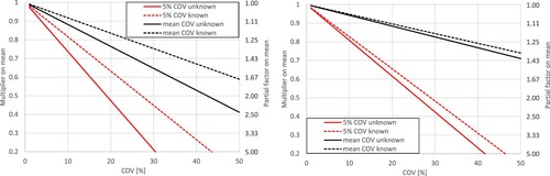
Table 1. Three-tier classification scheme of soil property variability for reliability calibration (Source: Table 9.7; Phoon and Kulhawy 2008).

Geotechnical parameter	Property variability	COV (%)
Undrained shear strength	Low^a	10–30
	Medium^b	30–50
	High^c	50–70
Effective stress friction angle	Low^a	5–10
	Medium^b	10–15
	High^c	15–20
Horizontal stress coefficient	Low^a	30–50
	Medium^b	50–70
	High^c	70–90

^a Typical of good quality direct lab or field measurements.

^b Typical of indirect correlations with good field data, except for the standard penetration test (SPT).

^c Typical of indirect correlations with SPT field data and with strictly empirical correlations.

Figure 4. Variation of k with respect to δ/L.

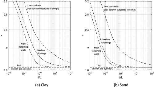
Figure 5. Statistics-based, mobilisation-based, and reliability-based characteristic values

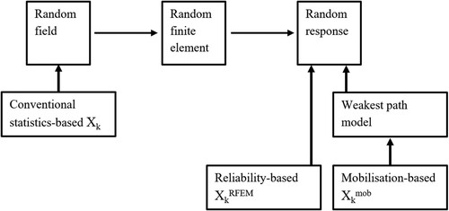
Table 2. Geotechnical resistance factors for the ultimate limit state (ULS) and serviceability limit state (SLS) appearing in Table 6.2 of the 2014 Canadian Highway Bridge Design Code (CHBDC) (CAN/CSAS614:2014). Numbers are for illustration only – the 2014 CHBDC must be consulted for the actual factors (Source: Table 4; Fenton et al. 2016).

Application	Limit State	Test Method/Model	Degree of understanding
			Low	Typical	High
Shallow foundations	Bearing, ${\phi }_{gu}$	Analysis	0.45	0.50	0.60
		Scale model test	0.50	0.55	0.65
	Sliding, ${\phi }_{gu}$ Frictional	Analysis	0.70	0.80	0.90
		Scale model test	0.75	0.85	0.95
	Sliding, ${\phi }_{gu}$ Cohesive	Analysis	0.55	0.60	0.65
		Scale model test	0.60	0.65	0.70
	Passive resistance, ${\phi }_{gu}$	Analysis	0.40	0.50	0.55
	Settlement or lateral movement, ${\phi }_{gs}$	Analysis	0.70	0.80	0.90
		Scale model test	0.80	0.90	1.00
Deep foundations	Compression, ${\phi }_{gu}$	Static analysis	0.35	0.40	0.45
		Static test	0.50	0.60	0.70
		Dynamic analysis	0.35	0.40	0.45
		Dynamic test	0.45	0.50	0.55
	Tension, ${\phi }_{gu}$	Static analysis	0.20	0.30	0.40
		Static test	0.40	0.50	0.60
	Lateral, ${\phi }_{gu}$	Static analysis	0.45	0.50	0.55
		Static test	0.45	0.50	0.55
	Settlement or lateral deflection, ${\phi }_{gs}$	Static analysis	0.70	0.80	0.90
		Static test	0.80	0.90	1.00
Ground Anchors	Pull-out, ${\phi }_{gu}$	Analysis	0.35	0.40	0.50
		Test	0.55	0.60	0.65
Internal MSE reinforcement	Rupture, ${\phi }_{gu}$	Analysis	0.75	0.80	0.85
		Test	0.85	0.90	0.95
	Pull-out, ${\phi }_{gu}$	Analysis	0.35	0.40	0.50
		Test	0.55	0.60	0.65
Retaining systems	Bearing, ${\phi }_{gu}$	Analysis	0.45	0.50	0.60
	Overturning, ${\phi }_{gu}$	Analysis	0.45	0.50	0.55
	Base sliding, ${\phi }_{gu}$	Analysis	0.70	0.80	0.90
	Facing interface sliding, ${\phi }_{gu}$	Test	0.75	0.85	0.95
	Connections, ${\phi }_{gu}$	Test	0.65	0.70	0.75
	Settlement, ${\phi }_{gs}$	Analysis	0.70	0.80	0.90
	Deflection/tilt, ${\phi }_{gs}$	Analysis	0.70	0.80	0.90
Embankments (fill)	Bearing, ${\phi }_{gu}$	Analysis	0.45	0.50	0.60
	Sliding, ${\phi }_{gu}$	Analysis	0.70	0.80	0.90
	Global stability-temporary, ${\phi }_{gu}$	Analysis	0.70	0.75	0.80
	Global stability-permanent, ${\phi }_{gu}$	Analysis	0.60	0.65	0.70
	Settlement, ${\phi }_{gs}$	Analysis	0.70	0.80	0.90
		Test	0.80	0.90	1.00

Table 3. Undrained uplift resistance/deformation factors for LRFD (Phoon, Kulhawy, and Grigoriu 2003a).

			Ψu
Depth/Width	Width (m)	COV of K (%)	Resistance factor (ULS)	Deformation factor (SLS)
1–2	1 – 2	30–50	0.45	0.69
		50–70	0.43	0.66
		70–90	0.41	0.63
	2 – 3	30–50	0.42	0.63
		50–70	0.40	0.60
		70–90	0.38	0.58
2–3	1 – 2	30–50	0.41	0.62
		50–70	0.38	0.58
		70–90	0.36	0.55
	2 – 3	30–50	0.39	0.58
		50–70	0.36	0.54
		70–90	0.34	0.51

Note: K = operative horizontal stress coefficient; target reliability index = 3.2 for resistance factors (ULS) and 2.6 for deformation factors (SLS)

Figure 6. In situ effective vertical stress (solid line), preconsolidation profile (dashed line), and final stress state (dotted line) for the settlement example. The square markers indicate the preconsolidation pressure values from the oedometer tests. The groundwater table at 1.5 m depth is indicated by a dashed dotted line.

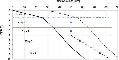
Table 4. Water content and the deformation properties obtained from oedometer tests.

Depth [m]	w [%]	σ’cv [kPa]	MOC [kPa]	m	a
2.5	90.8	50	1400	5.5	−1.1
4.2	118.1	50	1100	4.6	−1.2
6.2	116.8	58	1350	3.7	−1.5
8.7	85.9	75	2000	3.5	−1.35

Table 5. Combinations for simple statistical characteristic value calculations.

Set of characteristic values	n = 1	n = 4
Best estimate values, i.e. values presented in Table 4.	(X)	(X)
5% mean values for M and a		X
5% mean values for M and m		X
5% mean values for M, m, and a		X
5% mean values for σ’cv	X	X
5% mean values for σ’cv, M and m	X	X
5% mean values for σ’cv, M, m and a		X

Figure 7. Influence of number of samples a) and comparison of different sets of characteristic values for n = 4 b) to the ratio between characteristic and best estimate settlement.

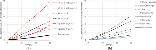
Figure 8. Reliability based characteristic settlement calculations. The influence of positive vs. negative correlation a), the influence of normal vs. log normal distributions b), comparison of RBD vs. ERD characteristic settlement calculations c) and comparison of simple static and RBD/ERD characteristic settlement calculations for n = 4.

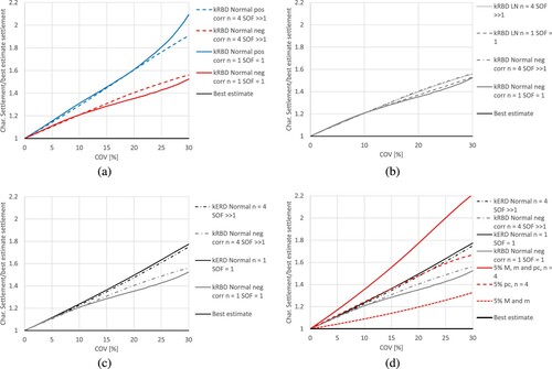
Table 6. Example of empirical deformation factors (herein defined as multipliers applied to best estimate settlement) depending on the level of understanding and consequence of exceeding the serviceability limit state.

			Consequence
			Low	Normal	High
			1	1.1	1.2
Level of understanding	High	1.1	1.1	1.21	1.32
	Normal	1.3	1.3	1.43	1.56
	Low	1.5	1.5	1.65	1.8

Figure 9. a) Resistance factors (Fenton et al. (2016) and b) partial factors (Länsivaara and Knuuti 2015) depending on the level of understanding and consequence of failure.

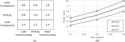
Table 7. Definition of Geotechnical Categories (GC) based on Consequence Classes (CC) and Geotechnical Complexity Classes (GCC) according to draft prEN-1997-1 (CEN 2020).

Consequence Class (CC)	Geotechnical Complexity Class (GCC)
	Lower (GCC1)	Normal (GCC2)	Higher (GCC3)
Higher (CC3)	GC2	GC3	GC3
Normal (CC2)	GC2	GC2	GC3
Lower (CC1)	GC1	GC2	GC2

Bond, A., and A. Harris. 2008. Decoding Eurocode 7. London: Taylor and Francis.

 Google Scholar

Phoon, K. K., and F. H. Kulhawy. 2008. Serviceability Limit State Reliability-based Design. Chapter 9, Reliability-Based Design in Geotechnical Engineering: Computations and Applications, Taylor & Francis, UK, 344–383.

 Google Scholar

CAN/CSAS614:2014. Canadian Highway Bridge Design Code. Mississauga, Ontario, Canada: Canadian Standards Organization.

 Google Scholar

Fenton, G. A., F. Naghibi, D. Dundas, R. J. Bathurst, and D. V. Griffiths. 2016. “Reliability-based Geotechnical Design in 2014 Canadian Highway Bridge Design Code.” Can. Geotech. J 53: 236–251. doi:https://doi.org/10.1139/cgj-2015-0158.

 Web of Science ®Google Scholar

Phoon, K. K., F. H. Kulhawy, and M. D. Grigoriu. 2003a. “Multiple Resistance Factor Design (MRFD) for Spread Foundations. Journal of Geotechnical and Geoenvironmental Engineering.” ASCE 129 (9): 807–818.

 Google Scholar

Länsivaara, T., and M. Knuuti. 2015. A Proposal for some Modifications of EN 1997-1 Design Approaches. in Fifth International Symposium on Geotechnical Safety and Risk (ISGSR): Rotterdam, The Netherlands 13–16 October 2015. IOS Press, pp. 486–491, International Symposium on Geotechnical Safety and Risk, Netherlands, 1/11/10.

 Google Scholar

CEN. 2020. prEN 1997-1 Geotechnical design – General rules (PT6) Oct2020. Comité Européen de Normalisation.

 Google Scholar