Figures & data
Figure 1. Urban charctaeristics of the case study suburbs in Western Sydne.
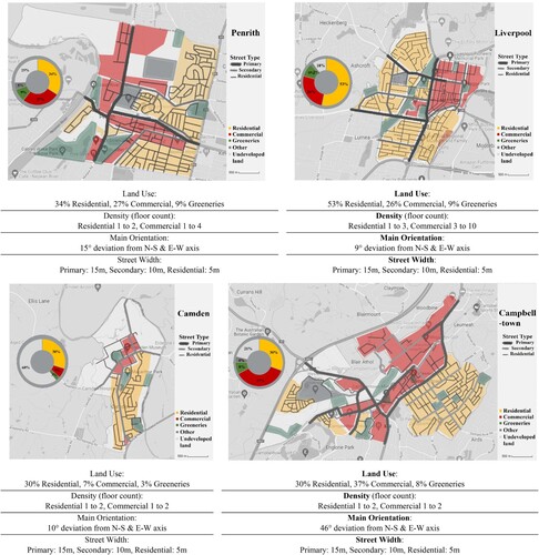
Figure 2. Computational simulation workflow.
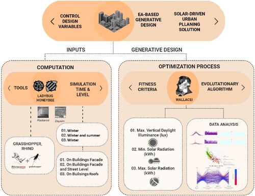
Figure 3. Developed Algorithm and the associated used tool in each step.
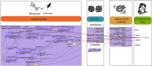
Figure 4. developed urban model.
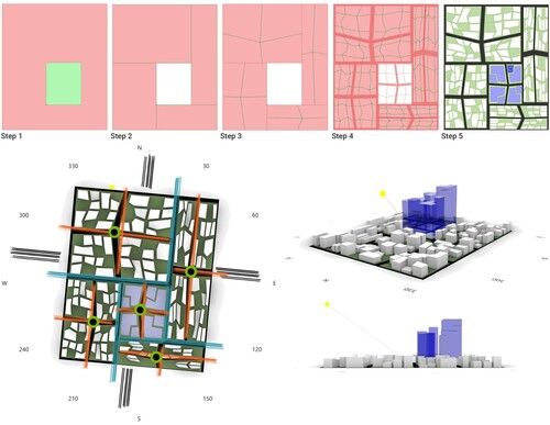
Figure 5. Simplified urban model (phenotypes) and the associated evaluation grid sensors (colored in red).
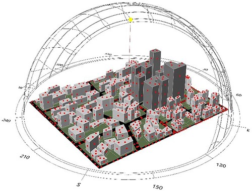
Table 1. Simulation settings.
Table 2. Influential design factors.
Figure 6. An example of Pareto-frontier based optimization (Image source: (Pilechiha et al., Citation2020)).
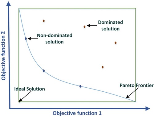
Figure 8. The relation between set fitness objective.
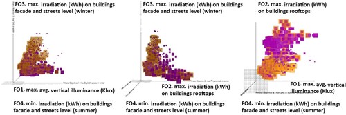
Figure 7. SD graph, fitness values, SD trendline, and mean value trend line for fitness objectives.
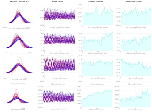
Figure 9. Parallel Coordinate Plots of the top-ranked individual for Fitness Average (top) and Relative Difference (bottom).
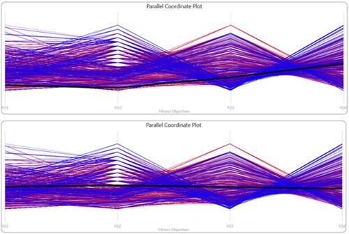
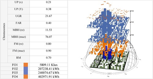
Table 3. Multi-responsive design scenarios using RD and FA methods and the utopia solution with their related genes, layouts, values, and chromosomes (from top to bottom).
Figure 10. Parallel coordinate plot (top) and unsupervised machine learning algorithm (bottom) of the Pareto Front solutions.
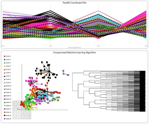
Figure 11. The outlier solutions.
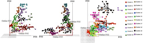
Figure 12. Optimum solution suggested by Evolutionary Method.
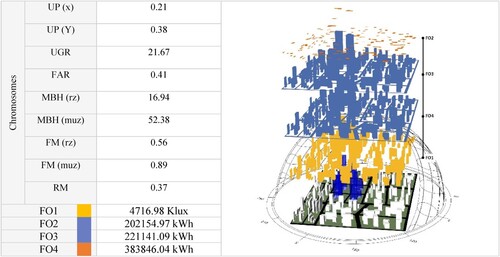
Table 4. Variable range of design parameters.
Table 5. Impact size of design parameters on different objectives
Figure 13. Improved solution suggested by the parametric approach.