Dynamic equilibria in an epidemic model with voluntary vaccinations†

^†Comments and suggestions from anonymous referees of the journal are gratefully acknowledged. This paper is dedicated to the loving memory of Lucy Hauser

Figures & data

Figure 1. The benefit and cost of vaccination as functions of the steady-state prevalence. The parameter values used are: β=1, δ=0.07, ϵ=0.8, u=100, and c=338. With the given parameter values, and p=0.62. The solutions to the equation B(p)=c are 0.78 and 0.036. Since there does not exist a solution to Equations (9)–(11) satisfying p=0.036 and α∈[0, 1], there cannot be an SSREE in which p=0.036. On the other hand, we obtain α=0.48∈[0, 1] from solving Equations (9)–(11) given p=0.78. Therefore there exists an SSREE with (α, p)=(0.48, 0.78).

Figure 2. The coexistence of multiple REEs starting with the same initial prevalence level. The parameter values used are: β=1, δ=0.07, ϵ=0.8, u=100, and c=338. Given initial prevalence p ₀=0.7 (and v ₀=0), there exists an REE in which α _t =0 ∀ t and p _t converges to ; there also exists an REE in which α _t =1 ∀ t and p _t converges to p=0.62.

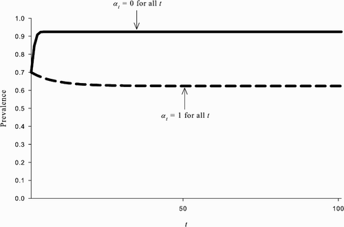
Figure 3. Assuming the population is initially at the no-vaccination steady state, there can exist an REE in which susceptible agents’ behaviour changes starting at time T and the population eventually reaches the all-vaccinate steady state.

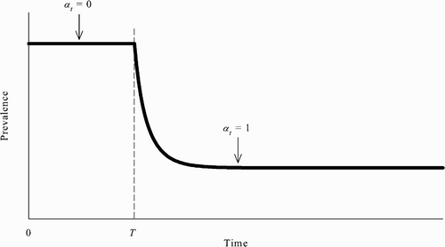
Figure 4. The net cost of vaccination at time t<T given and α _t =1 ∀ t≥T. The plot shows U*(p _t )−(W*(p _t )−c), t<T, where W* and U*, respectively, satisfy Equations (29) and (30), as a function of T−t. The parameter values used are: β=1, δ=0.07, ϵ=0.8, u=100, and c=338.

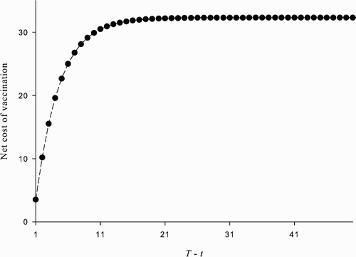
Figure 5. Assuming the population is initially at the all-vaccinate steady state, there can exist an REE in which susceptible agents’ behaviour changes starting at time T and the population eventually reaches the no-vaccination steady state.

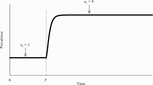
Figure 6. The net benefit of vaccination at time t<T given p _t =p ∀ t≤T and α _t =0 ∀ t≥T. The plot shows , t<T, where satisfies Equation (39), as a function of T−t. The parameter values used are: β=1, δ=0.07, ϵ=0.8, u=100, and c=338.

Figure 7. The existence of periodic REEs.

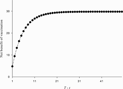
Figure 8. A plot of (solid line) and (dashed line) with respect to p, where and , respectively, solve Equations (43) and (44). The parameter values used are: β=1, δ=0.07, ϵ=0.8, u=100, and c=338.

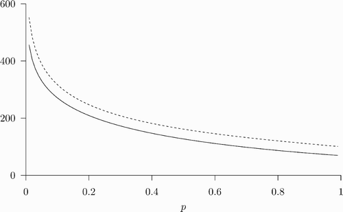
Figure 9. A plot of W (p)−c (solid line) and u+(1−δ) (1−β p) U (f(p)) (dashed line) with respect to p, where W solves Equation (49) and U satisfies Equation (50). The parameter values used are: β=1, δ=0.07, ϵ=0.8, u=100, and c=338. The two curves cross when p=0.0513 and p=0.973.

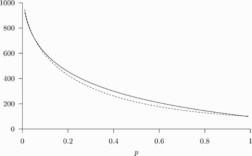
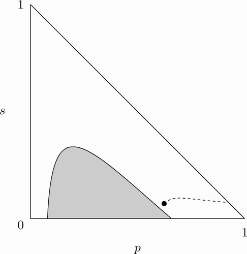
Figure 10. A comparison of U* *(p, s) and W* *(p, s)−c. The set of (p, s) such that U* *(p, s)>W* *(p, s)−c is indicated by the unshaded region, while the shaded region is the set of (p, s) at which U* *(p, s)≤W* *(p, s)−c. The point (p, s)=(p, δ) is indicated by the black dot. The parameter values used are: β=1, δ=0.07, ϵ=0.8, u=100, and c=338.