2,368
Views
37
CrossRef citations to date
0
Altmetric
Original Articles

Population collapse to extinction: the catastrophic combination of parasitism and Allee effect

Pages 86-101 | Received 06 Nov 2008, Published online: 17 Jun 2009

Figures & data

Figure 1. Phase plane illustrations with nullclines and stationary states of model (1) and (2). Solid (dashed) lines are the nullclines of infectives (total populations). Black (grey) points mark stable (unstable) equilibria. If the system is bistable (all panels except [e]), the stable manifolds of the saddle point separating the basins of attraction are shown in dotted lines. Parameter values: (a) μ=3.9, (b) μ=3.65, (c) μ=3, (d) μ=2.4, (e) μ=2, (f) μ=0.5 and β=4, u=0.1, r=2, d=0.2.

Figure 1. Phase plane illustrations with nullclines and stationary states of model (1) and (2). Solid (dashed) lines are the nullclines of infectives (total populations). Black (grey) points mark stable (unstable) equilibria. If the system is bistable (all panels except [e]), the stable manifolds of the saddle point separating the basins of attraction are shown in dotted lines. Parameter values: (a) μ=3.9, (b) μ=3.65, (c) μ=3, (d) μ=2.4, (e) μ=2, (f) μ=0.5 and β=4, u=0.1, r=2, d=0.2.

Figure 2. Bifurcation diagrams for varying basic reproduction number (by increasing β). Solid (dashed) lines correspond to stable (unstable) equilibria. The arrow indicates the abrupt population collapse from a level of a large population size N*+ after a saddle-node (SN) bifurcation. The critical values of ℛ0 are explained in the main text. Other parameter values: μ=1, u=0.1, r=2, d=0.2.
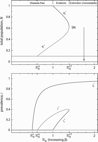
Figure 2. Bifurcation diagrams for varying basic reproduction number (by increasing β). Solid (dashed) lines correspond to stable (unstable) equilibria. The arrow indicates the abrupt population collapse from a level of a large population size N*+ after a saddle-node (SN) bifurcation. The critical values of ℛ0 are explained in the main text. Other parameter values: μ=1, u=0.1, r=2, d=0.2.

Figure 3. If the basic reproduction number is varied by changing pathogenicity, the bifurcation diagram reveals a second saddle-node bifurcation (SN2). Parameter values: β=4, u=0.1, r=2, d=0.2.
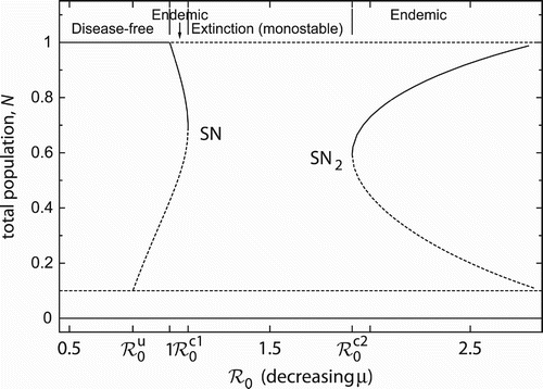
Figure 3. If the basic reproduction number is varied by changing pathogenicity, the bifurcation diagram reveals a second saddle-node bifurcation (SN2). Parameter values: β=4, u=0.1, r=2, d=0.2.

Figure 4. Domains of model behaviour in the two-parameter plane. Stable equilibria in each domain are indicated. The grey domain is monostable with eventual host extinction. All other domains are bistable. The hatched domain can be endemic, while the remaining white domains can be disease-free. Host extinction is always possible. Bold (thin) lines are saddle-node (transcritical) bifurcation curves. The dotted line marks the emergence of the unstable endemic equilibrium E . See the main text for more details. Parameter values: u=0.1, r=2, d=0.2.

Figure 4. Domains of model behaviour in the two-parameter plane. Stable equilibria in each domain are indicated. The grey domain is monostable with eventual host extinction. All other domains are bistable. The hatched domain can be endemic, while the remaining white domains can be disease-free. Host extinction is always possible. Bold (thin) lines are saddle-node (transcritical) bifurcation curves. The dotted line marks the emergence of the unstable endemic equilibrium E −. See the main text for more details. Parameter values: u=0.1, r=2, d=0.2.
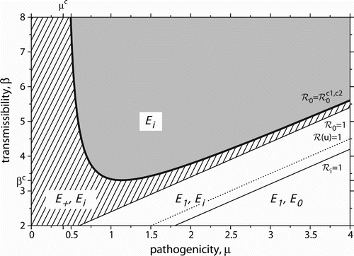
Figure 5. Time evolutions for varied basic reproduction numbers. (a), gradual transition from population persistence to extinction in the logistic model (8), (b) abrupt population collapse in the Allee effect model (2) when increasing ℛ0 (by increasing β), (c) decreasing ℛ0 (by varying μ) can lead to a population crash as well. Basic reproduction numbers are varied in equidistant steps. Initial conditions are fixed at N(t≡0)=1, i(t≡0)=0.01. Parameter values: μ=1, B=1, M=0.1 in the logistic model, u=0.1, r=2, d=0.2 in the Allee effect models with μ=1 (b) and β=4 (c).
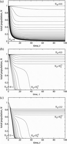
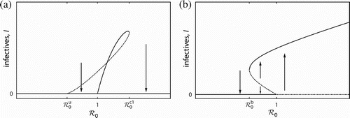
Figure 5. Time evolutions for varied basic reproduction numbers. (a), gradual transition from population persistence to extinction in the logistic model (8), (b) abrupt population collapse in the Allee effect model (2) when increasing ℛ0 (by increasing β), (c) decreasing ℛ0 (by varying μ) can lead to a population crash as well. Basic reproduction numbers are varied in equidistant steps. Initial conditions are fixed at N(t≡0)=1, i(t≡0)=0.01. Parameter values: μ=1, B=1, M=0.1 in the logistic model, u=0.1, r=2, d=0.2 in the Allee effect models with μ=1 (b) and β=4 (c).

Figure 6. (a) Bifurcation behaviour in the Allee effect model when varying ℛ0 by increasing β, (b) Stylized backward bifurcation. Note that the total host population goes extinct in (a) if the basic reproduction number is larger than . Parameter values in (a): μ=1, u=0.1, r=2, d=0.2, varying β.

Figure 6. (a) Bifurcation behaviour in the Allee effect model when varying ℛ0 by increasing β, (b) Stylized backward bifurcation. Note that the total host population goes extinct in (a) if the basic reproduction number is larger than . Parameter values in (a): μ=1, u=0.1, r=2, d=0.2, varying β.

Reprints and Corporate Permissions

Please note: Selecting permissions does not provide access to the full text of the article, please see our help page How do I view content?

To request a reprint or corporate permissions for this article, please click on the relevant link below:

Academic Permissions

Please note: Selecting permissions does not provide access to the full text of the article, please see our help page How do I view content?

Obtain permissions instantly via Rightslink by clicking on the button below:

If you are unable to obtain permissions via Rightslink, please complete and submit this Permissions form. For more information, please visit our Permissions help page.