716
Views
3
CrossRef citations to date
0
Altmetric
Original Articles

Dynamics of a discrete-time host–parasitoid system with cannibalism

&
Pages 419-435 | Received 09 Feb 2010, Accepted 28 Jul 2010, Published online: 17 Mar 2011

Figures & data

Figure 1. This figure provides simulation results for system Equation(1) with function g given in EquationEquation (26) and parameter values given in EquationEquation (27): (a) plots y=det(J(E 1)) against c; (b) provides a closed invariant curve solution when c=1.079; (c) is the bifurcation diagram with c as the bifurcation parameter; and (d) plots a particular solution when c=2.0, x 1(0)=2.0 and x 2(0)=3.0, where ‘.’ denotes x 1 and ‘-’ denotes x 2.
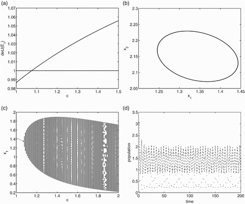
Figure 1. This figure provides simulation results for system Equation(1) with function g given in EquationEquation (26) and parameter values given in EquationEquation (27): (a) plots y=det(J(E 1)) against c; (b) provides a closed invariant curve solution when c=1.079; (c) is the bifurcation diagram with c as the bifurcation parameter; and (d) plots a particular solution when c=2.0, x 1(0)=2.0 and x 2(0)=3.0, where ‘.’ denotes x 1 and ‘-’ denotes x 2.

Figure 2. This figure provides simulation results for system Equation(17) with function g given in EquationEquation (26), f given in EquationEquation (28), and parameter values given in EquationEquation (29): (a) provides the time evolution of a particular solution when c=β=1.0; (b) presents the time evolution of a particular solution when c=1.0 and β=2.0; (c) plots the time evolution of a particular solution when c=2.0 and β=1.0; (d) provides a particular solution when c=2.0 and β=3.0. In all these plots, ‘.’ denotes x 1 and ‘*’ denotes p and initial conditions are (1, 1, 2) for each solution presented.
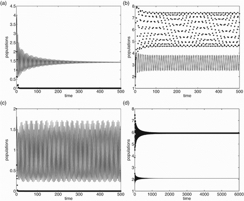
Figure 2. This figure provides simulation results for system Equation(17) with function g given in EquationEquation (26), f given in EquationEquation (28), and parameter values given in EquationEquation (29): (a) provides the time evolution of a particular solution when c=β=1.0; (b) presents the time evolution of a particular solution when c=1.0 and β=2.0; (c) plots the time evolution of a particular solution when c=2.0 and β=1.0; (d) provides a particular solution when c=2.0 and β=3.0. In all these plots, ‘.’ denotes x 1 and ‘*’ denotes p and initial conditions are (1, 1, 2) for each solution presented.

Reprints and Corporate Permissions

Please note: Selecting permissions does not provide access to the full text of the article, please see our help page How do I view content?

To request a reprint or corporate permissions for this article, please click on the relevant link below:

Academic Permissions

Please note: Selecting permissions does not provide access to the full text of the article, please see our help page How do I view content?

Obtain permissions instantly via Rightslink by clicking on the button below:

If you are unable to obtain permissions via Rightslink, please complete and submit this Permissions form. For more information, please visit our Permissions help page.