Effect of resource subsidies on predator–prey population dynamics: a mathematical model

Figures & data

Figure 1. Outcome of (a) the predator–prey model (I) for different carrying capacities k and (b) the predator-subsidy model (II) for different subsidy input rates i.

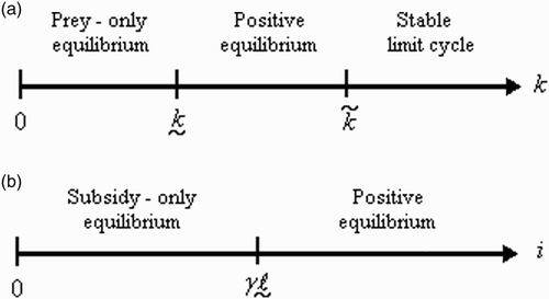
Table 1. Equilibrium properties of the predator–prey model (I).

Equilibrium	x*	y*	Feasible	Stable (when feasible)
Trivial	0	0	Always	Never
Prey-only	k	0	Always
Positive
^aA stable limit cycle occurs when k>[ktilde].

Table 2. Equilibrium properties of the predator-subsidy model (II).

Equilibrium	s*	y*	Feasible	Stable (when feasible)
Subsidy-only	i/γ	0	Always
Positive				Always

Figure 2. Time-series for the non-spatial predator–prey-subsidy model (III) with the following parameter values: r=0.1, θ=5, e=1, γ=1, ψ=5, ε=0.1, η=0.1, and δ=0.1. In (a) the prey population size approaches a positive equilibrium value, the subsidy amount approaches its natural value, and the predator becomes extinct (k=0.1 and i=0.12). In (b) the prey becomes extinct, the subsidy amount approaches its natural value, and the predator population size approaches a positive equilibrium value (k=0.1 and i=0.3). In (c) the predator and prey population sizes approach positive equilibrium values and the subsidy amount approaches its natural value (k=0.4 and i=0.2). In (d) the predator, prey, and subsidy all persist in a stable limit cycle (k=2 and i=0.05). In all figures, x(0)=0.2, y(0)=0.1, s(0)=0, k =0.25, and ℓ=0.25.

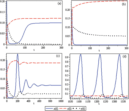
Table 3. Equilibrium properties of the predator–prey-subsidy model (III).

Equilibrium	x*	s*	y*	Feasible	Stable (when feasible)
Subsidy-only	0	i/γ	0	Always	Never
Predator-free	k	i/γ	0	Always	and i<i *(k)
Prey-free	0				i>i*
Positive	x*	s*	y*	and	Always^a
				and i<i*	Always^a
				k>[ktilde] and i<i*
Note: The quantities k , , i *(k), and i* are defined in Equations (2), (4), and (6).
^aConjecture.
^bLimit cycles (or other non-equilibrium dynamics) are conjectured to occur when i<i **(k).

Figure 3. Outcome of the non-spatial predator–prey-subsidy model (III) for different values of the carrying capacity (k) and subsidy input rate (i) based on local stability analysis. The system moves to a predator-free equilibrium in the lower-left region (red), to a prey-free equilibrium in the upper region (yellow), to a positive equilibrium in the central region (green), and to a stable limit cycle involving predator, prey, and subsidy in the lower-right region (blue). The lower-left boundary is given by i=i _*(k), the upper boundary is given by i=i*, and the lower-right boundary is given by i=i _**(k). All results are theoretical except for the stability of the positive equilibrium in the central and lower-right regions which is based instead on numerical evidence. The parameter values used are the same as in Figure 2.

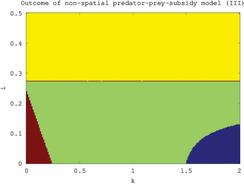
Figure 4. Time-series for the spatial predator–prey-subsidy model (IV) with the following parameter values: r=0.1, θ=5, a=1, γ=1, ψ=5, c=1, ε=0.1, η=0.1, δ=0.1, and α=0.8. In (a) the prey population size approaches a positive equilibrium value, the subsidy amount approaches its natural value, and the predator becomes extinct (k=0.1 and i=0.1). In (b) the prey becomes extinct, the subsidy amount approaches its natural value, and the predator population sizes approach positive equilibrium values (k=0.1 and i=1.0). In (c) the predator and prey population sizes approach positive equilibrium values and the subsidy amount approaches its natural value (k=0.4 and i=0.3). In (d) the predator, prey, and subsidy all persist in a stable limit cycle (k=2.4 and i=0.1). In all figures, x(0)=0.2, y ₁(0)=0.1, y ₂(0)=0, s(0)=0, k (α)=0.25, and ℓ(α)=0.65.

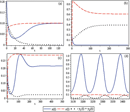
Table 4. Equilibrium properties of the spatial predator–prey-subsidy model (IV).

Equilibrium	x*	s*			Feasible	Stable (when feasible)
Subsidy-only	0	i/γ	0	0	Always	Never
Predator-free	k	i/γ	0	0	Always	and
Prey-free	0
Positive	x*	s*			and	Always ^a
					and	Always ^a
					and	^a, b
Notes: The quantities , , , and i*(α) are defined in Equations (19)–(22). All statements involving the positive equilibrium assume that and are finite and that is infinite.
^aConjecture.
^bLimit cycles (or other non-equilibrium dynamics) are conjectured to occur when .

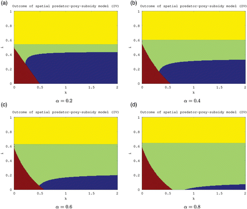
Figure 5. Outcome of the spatial predator–prey-subsidy model (IV) for different values of the carrying capacity (k), subsidy input rate (i), and predator-movement rate (α) based on local stability analysis. The system moves to a predator-free equilibrium in the lower-left region (red), to a prey-free equilibrium in the upper region (yellow), to a positive equilibrium in the central region (green), and to a stable limit cycle involving predator, prey, and subsidy in the lower-right region (blue). The lower-left boundary is given by i=i _*(k,α), the upper boundary is given by i=i*(α), and the lower-right boundary is given by i=i _**(k,α). The lower-left and upper boundaries both increase as α increases. All results are theoretical except for the stability of the positive equilibrium in the central and lower-right regions which is based instead on numerical evidence. The parameter values used are the same as in Figure 4 unless noted otherwise.