638
Views
7
CrossRef citations to date
0
Altmetric
Original Articles

Responses of the haploid-to-diploid ratio of isomorphic biphasic life cycles to time instability

&
Pages 1067-1087 | Received 08 Sep 2011, Accepted 13 Aug 2012, Published online: 20 Sep 2012

Figures & data

Figure 1. Overall persistence rate (colour scale) plotted upon the triangular ordination of the λ elasticities to fertility (F), growth (G) and looping (L). The coordinate of a point in each axis is given by a line parallel to the lines that intercept the axis coming from its right side.
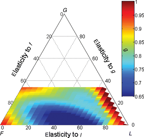
Figure 1. Overall persistence rate (colour scale) plotted upon the triangular ordination of the λ elasticities to fertility (F), growth (G) and looping (L). The coordinate of a point in each axis is given by a line parallel to the lines that intercept the axis coming from its right side.

Figure 2. Persistence rates (colour scale) of the specified sets plotted upon the triangular ordination of the λ elasticities to F, G and L. The coordinate in each axis is given by a line parallel to the lines that intercept the axis coming from its right side. (a) Real and equal set, (b) real and symmetric set, (c) complex conjugate and equal set and (d) complex conjugate and symmetric set. The (a) with (n) a negative eigenvalue and (p) a positive eigenvalue.
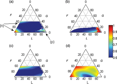
Figure 2. Persistence rates (colour scale) of the specified sets plotted upon the triangular ordination of the λ elasticities to F, G and L. The coordinate in each axis is given by a line parallel to the lines that intercept the axis coming from its right side. (a) Real and equal set, (b) real and symmetric set, (c) complex conjugate and equal set and (d) complex conjugate and symmetric set. The (a) with (n) a negative eigenvalue and (p) a positive eigenvalue.

Figure 3. Real equal set with a negative eigenvalue. In (a–c), the black solid line represents haploids and the blue dotted line represents diploids. The bias in each size class was standardized to the bias in the spores. In (e), the black lines represent haploids, the blue lines represent diploids, the solid lines represent the central tendency given by the dominant set and the dotted lines represent the linear combination of the dominant set and the real and equal set.
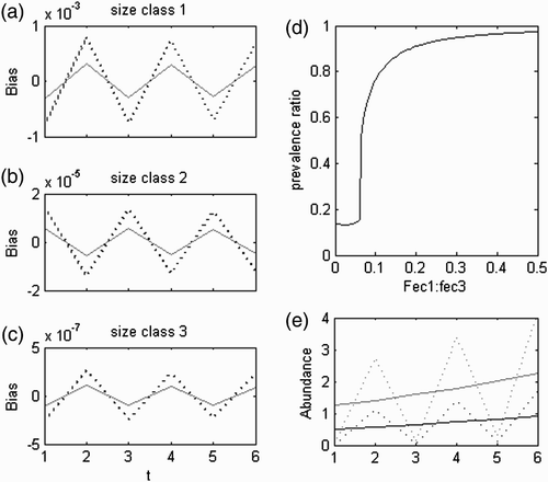
Figure 3. Real equal set with a negative eigenvalue. In (a–c), the black solid line represents haploids and the blue dotted line represents diploids. The bias in each size class was standardized to the bias in the spores. In (e), the black lines represent haploids, the blue lines represent diploids, the solid lines represent the central tendency given by the dominant set and the dotted lines represent the linear combination of the dominant set and the real and equal set.

Figure 4. Trajectory of the linear combination of the real symmetric sets. Simulation in the looping domain with i=−3.8, g=0.05 and l=0.96. Dissimilar L with d L =0.9. λ b a =0.88, λ c a =0.76, λ d a =0.67. γ a /∑ γ i =0.095, γ b /∑ γ i =0.093, γ c /∑ γ i =0.172, γ d /∑ γ i =0.253.

Figure 4. Trajectory of the linear combination of the real symmetric sets. Simulation in the looping domain with i=−3.8, g=0.05 and l=0.96. Dissimilar L with d L =0.9. λ b /λ a =0.88, λ c /λ a =0.76, λ d /λ a =0.67. γ a /∑ γ i =0.095, γ b /∑ γ i =0.093, γ c /∑ γ i =0.172, γ d /∑ γ i =0.253.
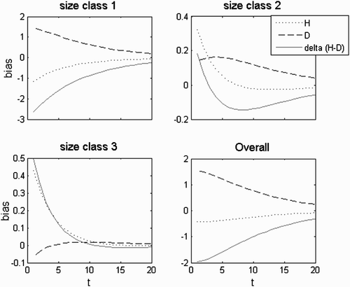
Figure 5. Bias to the central tendency given by the complex conjugate equal pair of eigenvectors, eigenvalues and c coefficients. Simulation in the growth domain with i=−3, g=0.8 and l=0. This was the demographic matrix with the highest elasticity to G. Dissimilar G with d G =0.8. Persistence rate=0.84.
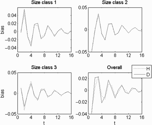
Figure 5. Bias to the central tendency given by the complex conjugate equal pair of eigenvectors, eigenvalues and c coefficients. Simulation in the growth domain with i=−3, g=0.8 and l=0. This was the demographic matrix with the highest elasticity to G. Dissimilar G with d G =0.8. Persistence rate=0.84.

Figure 6. Polar plots of the complex conjugate equal pair of eigenvectors and eigenvalues. In the eigenvalue are plotted λ b and θ b , whereas in size class ‘i’ are plotted σ i and ω i in red and σ i+4 and ω i+4 in blue. Simulation in the growth domain with i=−3, g=0.8 and l=0. Dissimilarities tested for d G from 1 to 0.6 at intervals of 0.02.
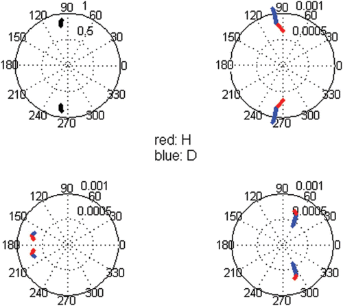
Figure 6. Polar plots of the complex conjugate equal pair of eigenvectors and eigenvalues. In the eigenvalue are plotted λ b and θ b , whereas in size class ‘i’ are plotted σ i and ω i in red and σ i+4 and ω i+4 in blue. Simulation in the growth domain with i=−3, g=0.8 and l=0. Dissimilarities tested for d G from 1 to 0.6 at intervals of 0.02.

Figure 7. Bias to the central tendency given by the complex conjugate symmetric pair of eigenvectors, eigenvalues and c coefficients. Simulation in the growth domain with i=−3, g=0.8 and l=0.01. This was the accepted demographic matrix with the higher elasticity to G. Dissimilar G with d G =0.8. Persistence rate= 0.95.
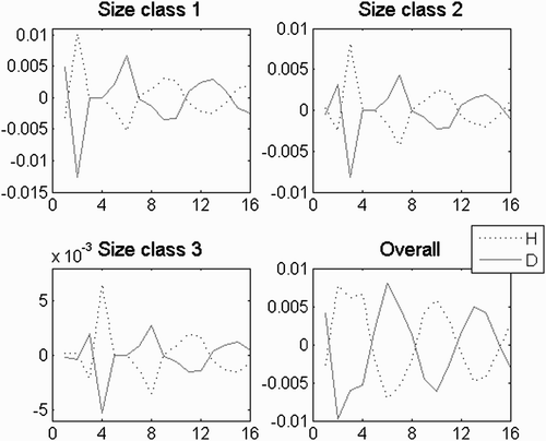
Figure 7. Bias to the central tendency given by the complex conjugate symmetric pair of eigenvectors, eigenvalues and c coefficients. Simulation in the growth domain with i=−3, g=0.8 and l=0.01. This was the accepted demographic matrix with the higher elasticity to G. Dissimilar G with d G =0.8. Persistence rate= 0.95.

Figure 8. H:D transient trajectories with the life strategy in (a) fertility domain with i=−2, g=0.08, l=0.05, d F =0.5, d G =1, d L =1; (b) growth domain with i=−3, g=0.8, l=0.01, d F =1, d G =0.8, d L =1; (c) looping domain with i=−3.8, g=0.8, l=0.96, d F =1, d G =1, d L =0.95, d spore=4, d 1=4, d 2=4 and d 3=4; (d) between the fertility and the growth domain with i=−2.5, g=0.5, l=0, d F =0.5, d G =0.5, d L =1; (e) between the fertility and the looping domain with i=−2.5, g=0.05, l=0.5, d F =2, d G =1, d L =0.7; and (f) between the growth and the looping domain with i=−3, g=0.3, l=0.5, d F =1, d G =1.5, d L =0.7.
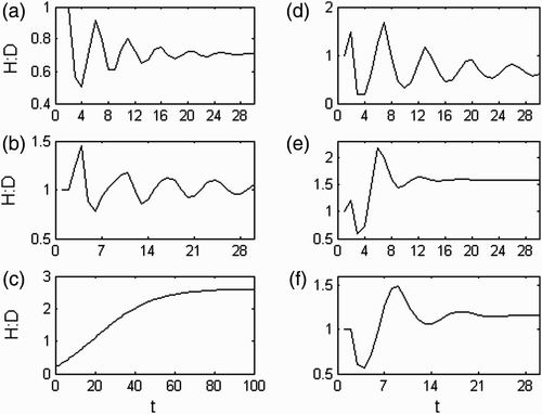
Figure 8. H:D transient trajectories with the life strategy in (a) fertility domain with i=−2, g=0.08, l=0.05, d F =0.5, d G =1, d L =1; (b) growth domain with i=−3, g=0.8, l=0.01, d F =1, d G =0.8, d L =1; (c) looping domain with i=−3.8, g=0.8, l=0.96, d F =1, d G =1, d L =0.95, d spore=4, d 1=4, d 2=4 and d 3=4; (d) between the fertility and the growth domain with i=−2.5, g=0.5, l=0, d F =0.5, d G =0.5, d L =1; (e) between the fertility and the looping domain with i=−2.5, g=0.05, l=0.5, d F =2, d G =1, d L =0.7; and (f) between the growth and the looping domain with i=−3, g=0.3, l=0.5, d F =1, d G =1.5, d L =0.7.

Figure A1. A(a) λ trajectory; (b) H:D trajectory; λ a =1.042; λ b, c =0.218±0.869i; abs(λ b, c )=0.9; θ b, c =±1.325 rad=±75.9°; wave period=4.74; persistence rate= 0.86.
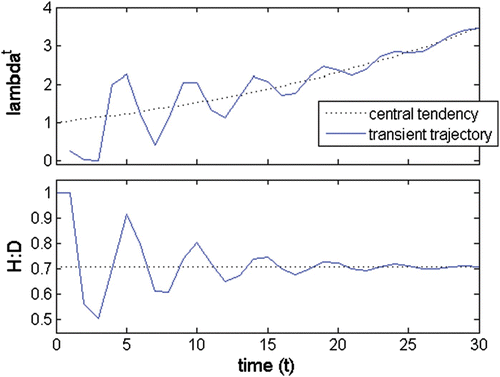
Figure A1. A(a) λ trajectory; (b) H:D trajectory; λ a =1.042; λ b, c =0.218±0.869i; abs(λ b, c )=0.9; θ b, c =±1.325 rad=±75.9°; wave period=4.74; persistence rate= 0.86.

Figure A2 Oscillatory trajectory of a strictly real negative eigenvalue; λ b =−0.68; θ b =180°; wave period= 2.
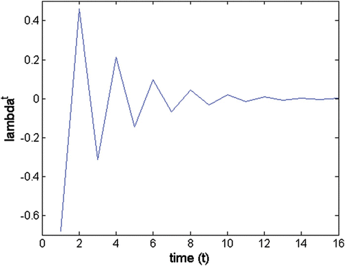
Figure A2 Oscillatory trajectory of a strictly real negative eigenvalue; λ b =−0.68; θ b =180°; wave period= 2.

Figure A3 Oscillatory trajectory of (left) a complex eigenvalue; λ b =0.598+0.679i; abs(λ b )=0.905; θ=48.6°; wave period=7.41 and (right) the complex conjugated pair of eigenvalues λ b and λ c .
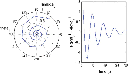
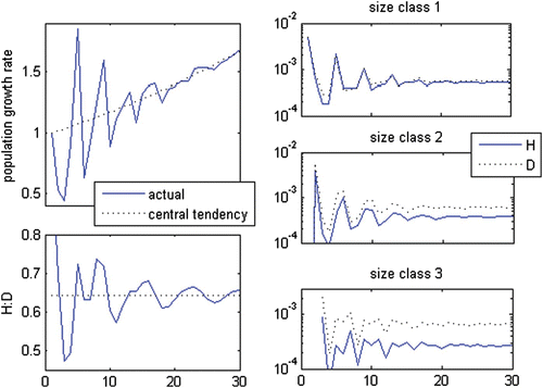
Figure A3 Oscillatory trajectory of (left) a complex eigenvalue; λ b =0.598+0.679i; abs(λ b )=0.905; θ=48.6°; wave period=7.41 and (right) the complex conjugated pair of eigenvalues λ b and λ c .
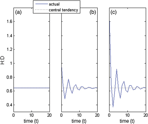
Figure A4 Eigval a =1.02, λ a =1.02 and θ a =0. Eigval b, c =−0.07±0.83i, λ b, c =0.83, persistence rate bc =0.81, θ b, c =±95.1° and wave period (b, c)=3.79; eigval d =−0.85, λ d =0.85, persistence rate bc =0.83, θ d =180° and wave period (d)=2.

Figure A4 Eigval a =1.02, λ a =1.02 and θ a =0. Eigval b, c =−0.07±0.83i, λ b, c =0.83, persistence rate bc =0.81, θ b, c =±95.1° and wave period (b, c)=3.79; eigval d =−0.85, λ d =0.85, persistence rate bc =0.83, θ d =180° and wave period (d)=2.

Figure A5 H:D when the c coefficients for the complex conjugated pair were multiplied (a) by 0, (b) by 1 and (c) by 2.

Figure A5 H:D when the c coefficients for the complex conjugated pair were multiplied (a) by 0, (b) by 1 and (c) by 2.