Heterogeneity in multiple transmission pathways: modelling the spread of cholera and other waterborne disease in networks with a common water source

Figures & data

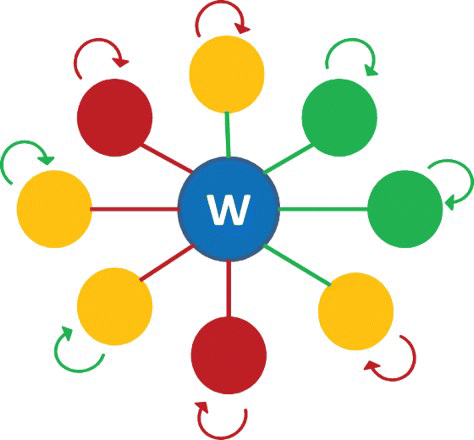
Figure 1. Schematic of metapopulation model: multiple patches and common water source W.\newline Note: Outer arrows represent within patch direct transmission, with red denoting high transmission rates and green low transmission rates. Spokes connecting patches to the shared water source are similarly coloured to represent levels of indirect transmission. Individual patches may have high (low) rates of transmission for both transmission pathways, and are coloured red (green) accordingly. Patches may also have high rates for one type of transmission and low rates for the other; these patches are coloured orange.

Figure 2. Schematic of 2-patch model.

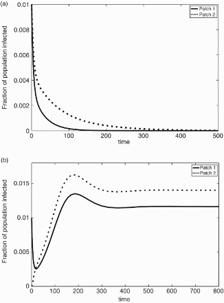
Figure 3. (a) R₀=0.7407 in patch 1, and R₀=0.9259 in patch 2. The disease dies out in both patches when each patch has its own water source. Patch 1 parameter values: β_W=0.1, β_I=0.1, γ=0.25, ξ=0.1. Patch 2 parameter values: β_W=0.1, β_I=0.15, γ=0.25, ξ=0.1. Initial conditions: 99% of the population susceptible and 1% infected in each patch. (b) R₀=1.2151 for two patch system with shared water source. The disease persists in both patches. 2-patch parameter values: , , , a₁=a₂=0.5, γ=0.25, ξ=0.1. Initial condition: 99% of the population in patch 1 susceptible and 1% infected; patch 2 100% susceptible.

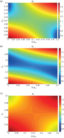
Figure 4. R₀ for model (4) as a function of distribution of both types of transmission across patches, for three cases: pathways contribute equally (), direct transmission dominates (, ), and indirect transmission dominates (, ). Axes denote the amount of transmission placed on patch 1, with the remainder placed on patch 2. For all cases, μ=0.02 and γ=0.25. (a) Direct and indirect transmission equal, (b) direct transmission dominant, and (c) indirect transmission dominant.

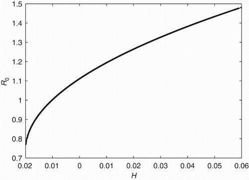
Figure 5. R₀ versus H, where H=var(β_I)+2 cov(a β_W, β_I), for 2-patch system, {with parameters as in Figure 4(a)}. R₀ is an increasing function of heterogeneity. This measure of heterogeneity incorporating the trade-off between different types of transmission is predictive of R₀.

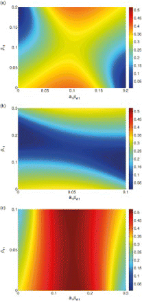
Figure 6. Shown are the total outbreak size (z₁+z₂) as a function of the distribution of transmission for three cases: direct and indirect transmission equal ( and , direct transmission dominant ( and ), and indirect transmission dominant ( and ). Axes denote the amount of each type of transmission on patch 1. Here μ=0 and γ=0.25. (a) Direct and indirect transmission equal, (b) direct transmission dominant, and (c) indirect transmission dominant.

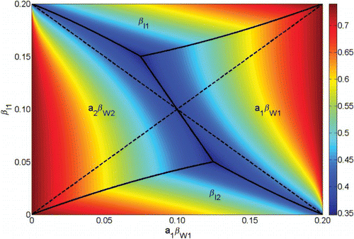
Figure 7. A comparison of the regions where the sensitivity of R₀ to each transmission parameter is greatest and the regions where each transmission parameter is greatest. Shown in colour is max((∂ R₀/∂ p)p) for , , , . The plane is divided into four regions (upper, lower, left, right) where R₀ is most sensitive to , , , and , respectively (boundaries denoted with solid black lines) and where each the value of each transmission parameter is greatest (boundaries denoted with dashed black lines). Here μ=0.02 and γ=0.25.

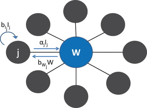
Figure 8. Schematic of n-patch setup with shared water source.

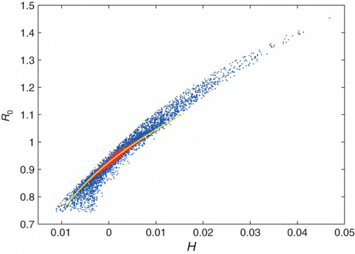
Figure 9. R₀ versus H (defined as H=var(β_I)+n cov(a β_W, β_I)) for a 4 patch network with a common water source, with both total water and person–person transmission held constant (, {μ=0.02, γ=0.25}). Shown are results from three simulations. First, transmission values for each patch are drawn from a complete random sampling of β_I, a β_W space (blue points). Next, all transmission values are restricted to symmetric perturbations from the average transmission rates (red points). Third, transmission parameters for each patch only have two possible values, high or low, and these values are determined by a random perturbation from the average transmission rate (yellow curve).