4,992
Views
14
CrossRef citations to date
0
Altmetric
Original Articles

A comparison of a deterministic and stochastic model for Hepatitis C with an isolation stage

, , &
Pages 276-301 | Received 14 Nov 2012, Accepted 19 Oct 2013, Published online: 19 Nov 2013

Figures & data

Figure 1. Flow diagram of the model (1). The model consists of five sub-populations: susceptible S, acute A, chronic C, isolated Q and recovered R individuals.
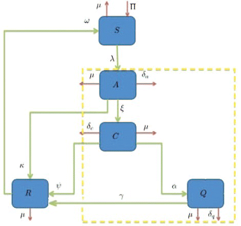
Figure 1. Flow diagram of the model (1). The model consists of five sub-populations: susceptible S, acute A, chronic C, isolated Q and recovered R individuals.

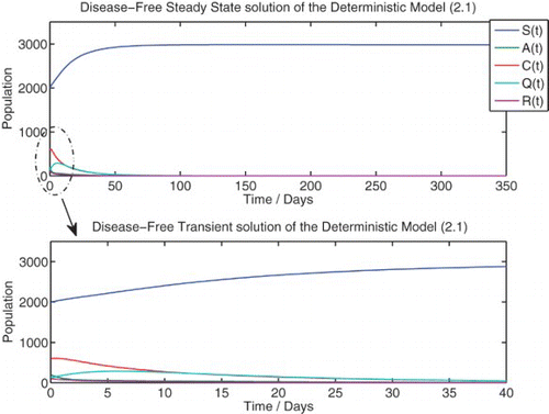
Figure 2. Numerical solution of the deterministic model (1) at {R0=0.6453}. Initial population:

Π=0.12; γ=0.18; κ=0.2; ω=0.95;
ξ=0.7; α=0.15; ψ=0.05; δa=0.000233; δc=0.00233; δq=0.001667; η=0.5; ζ=0.1; β=0.1369.

Figure 2. Numerical solution of the deterministic model (1) at {R0=0.6453}. Initial population: Display full size Π=0.12; γ=0.18; κ=0.2; ω=0.95; Display full size ξ=0.7; α=0.15; ψ=0.05; δa=0.000233; δc=0.00233; δq=0.001667; η=0.5; ζ=0.1; β=0.1369.

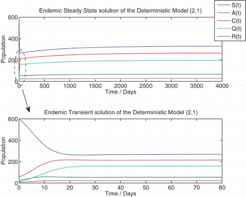
Figure 3. Numerical solution of the deterministic model (1) at {R0=2.6889}. Initial population: (

(0),
(0),
(0),
(0),
(0))=(600, 20, 60, 12, 10). Π=1; γ=0.18; κ=0.2; ω=0.95;
ξ=0.7; α=0.15; ψ=0.05; δa=0.000233; δc=0.00233; δq=0.001667; η=0.5; ζ=0.1; β=0.5703.

Figure 3. Numerical solution of the deterministic model (1) at {R0=2.6889}. Initial population: (Display full size(0), Display full size(0), Display full size(0), Display full size(0), Display full size(0))=(600, 20, 60, 12, 10). Π=1; γ=0.18; κ=0.2; ω=0.95; Display full size ξ=0.7; α=0.15; ψ=0.05; δa=0.000233; δc=0.00233; δq=0.001667; η=0.5; ζ=0.1; β=0.5703.

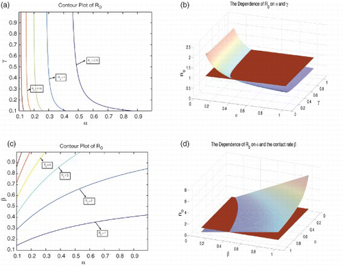
Figure 4. The dependence of R0 on some state variables. (a) The contour plot of R0 as a function of α and γ, (b) R0 as a function of α and γ, (c) the contour plot of R0 as a function of α and β and (d) R0 as a function of α and β. Π=10; γ=0.1; κ=0.7535; ω=0.95;

ξ=0.8; α=0.2; ψ=0.05; δa=0.000233; δc=0.00233; δq=0.001667; η=0.5; ζ=0.1; β=0.3.

Figure 4. The dependence of R0 on some state variables. (a) The contour plot of R0 as a function of α and γ, (b) R0 as a function of α and γ, (c) the contour plot of R0 as a function of α and β and (d) R0 as a function of α and β. Π=10; γ=0.1; κ=0.7535; ω=0.95; Display full size ξ=0.8; α=0.2; ψ=0.05; δa=0.000233; δc=0.00233; δq=0.001667; η=0.5; ζ=0.1; β=0.3.

Figure 5. Comparison of the solution to the deterministic model (1) and the numerical means of each discrete random variable from the stochastic model at R0=2.6889.
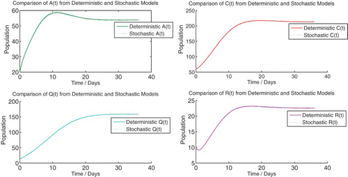
Figure 5. Comparison of the solution to the deterministic model (1) and the numerical means of each discrete random variable from the stochastic model at R0=2.6889.

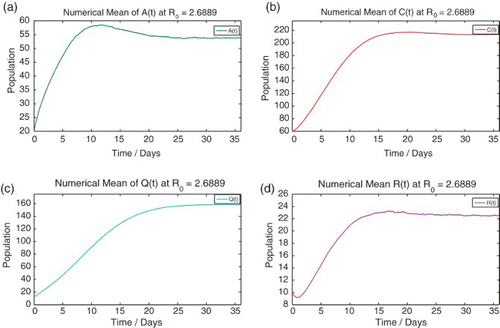
Figure 6. The numerical mean of each discrete random variable calculated using 10,000 sample paths. Numerical mean of the discrete random variables (a)

(t), (b)
(t), (c)
(t) and (d)
(t). Initial population: (
(0),
(0),
(0),
(0),
(0))=(600, 20, 60, 12, 10). Π=1; γ=0.18; κ=0.2; ω=0.95;
ξ=0.7; α=0.15; ψ=0.05; δa=0.000233; δc=0.00233; δq=0.001667; η=0.5; ζ=0.1; β=0.5703.

Figure 6. The numerical mean of each discrete random variable calculated using 10,000 sample paths. Numerical mean of the discrete random variables (a) Display full size(t), (b) Display full size(t), (c) Display full size(t) and (d) Display full size(t). Initial population: (Display full size(0), Display full size(0), Display full size(0), Display full size(0), Display full size(0))=(600, 20, 60, 12, 10). Π=1; γ=0.18; κ=0.2; ω=0.95; Display full size ξ=0.7; α=0.15; ψ=0.05; δa=0.000233; δc=0.00233; δq=0.001667; η=0.5; ζ=0.1; β=0.5703.

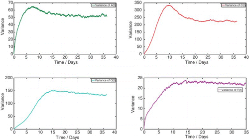
Figure 7. The variance of each discrete random variable calculated using 10,000 sample paths: (a)

(t), (b)
(t), (c)
(t) and (d)
(t).

Figure 7. The variance of each discrete random variable calculated using 10,000 sample paths: (a) Display full size(t), (b) Display full size(t), (c) Display full size(t) and (d) Display full size(t).

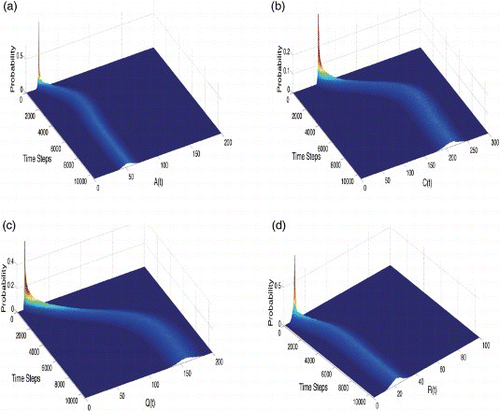
Figure 8. The probability distribution of each discrete random variable calculated using 5000 sample paths. (a) Probability distribution of

(t) at {R0=2.6889}, (b) probability distribution of
(t) at {R0=2.6889}, (c) probability distribution of
(t) at {R0=2.6889} and (d) probability distribution of
(t) at {R0=2.6889}. Initial population: (
(0),
(0),
(0),
(0),
(0))=(600, 20, 60, 12, 10). Π=1; γ=0.18; κ=0.2; ω=0.95;
ξ=0.7; α=0.15; ψ=0.05; δa=0.000233; δc=0.00233; δq=0.001667; η=0.5; ζ=0.1; β=0.5703.

Figure 8. The probability distribution of each discrete random variable calculated using 5000 sample paths. (a) Probability distribution of Display full size(t) at {R0=2.6889}, (b) probability distribution of Display full size(t) at {R0=2.6889}, (c) probability distribution of Display full size(t) at {R0=2.6889} and (d) probability distribution of Display full size(t) at {R0=2.6889}. Initial population: (Display full size(0), Display full size(0), Display full size(0), Display full size(0), Display full size(0))=(600, 20, 60, 12, 10). Π=1; γ=0.18; κ=0.2; ω=0.95; Display full size ξ=0.7; α=0.15; ψ=0.05; δa=0.000233; δc=0.00233; δq=0.001667; η=0.5; ζ=0.1; β=0.5703.

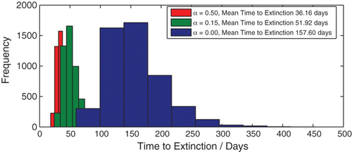
Figure 9. Mean time to disease extinction plotted as a histogram for three cases: α=0, α=0.15 and α=0.5. Initial population: (

(0),
(0),
(0),
(0),
(0))=(600, 20, 60, 10, 10). Π=1; γ=0.2; κ=0.2; ω=0.95;
ξ=0.8; ψ=0.05; δa=0.000233; δc=0.00233; δq=0.001667; η=0.5; ζ=0.1; β=0.1880; Δ t=0.0069.

Figure 9. Mean time to disease extinction plotted as a histogram for three cases: α=0, α=0.15 and α=0.5. Initial population: (Display full size(0), Display full size(0), Display full size(0), Display full size(0), Display full size(0))=(600, 20, 60, 10, 10). Π=1; γ=0.2; κ=0.2; ω=0.95; Display full size ξ=0.8; ψ=0.05; δa=0.000233; δc=0.00233; δq=0.001667; η=0.5; ζ=0.1; β=0.1880; Δ t=0.0069.

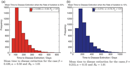
Figure 10. The mean time to disease extinction for two cases in which the basic reproduction number R0 is slightly greater than unity computed using 5000 stochastic simulations each. Mean time to disease extinction for the cases (a) β=0.439,α=0.50 and R0=1.01 and (b) β=0.213,α=0.15 and R0=1.01. Initial population: (

(0),
(0),
(0),
(0),
(0))=(600, 20, 60, 10, 10). Π=1; γ=0.2; κ=0.2; ω=0.95;
ξ=0.8; ψ=0.05; δa=0.000233; δc=0.00233; δq=0.001667; η=0.5; ζ=0.1; Δ t=0.0069.

Figure 10. The mean time to disease extinction for two cases in which the basic reproduction number R0 is slightly greater than unity computed using 5000 stochastic simulations each. Mean time to disease extinction for the cases (a) β=0.439,α=0.50 and R0=1.01 and (b) β=0.213,α=0.15 and R0=1.01. Initial population: (Display full size(0), Display full size(0), Display full size(0), Display full size(0), Display full size(0))=(600, 20, 60, 10, 10). Π=1; γ=0.2; κ=0.2; ω=0.95; Display full size ξ=0.8; ψ=0.05; δa=0.000233; δc=0.00233; δq=0.001667; η=0.5; ζ=0.1; Δ t=0.0069.