Cell cycle dynamics in a response/signalling feedback system with a gap

Figures & data

Fig. 1. An illustration of the map F with k=3; F(x₂, x₃)=(x′₂, x′₃).

Fig. 2. Return map F for Case I when α=0.5, s=0.2, r=0.6, and ε=0.05.

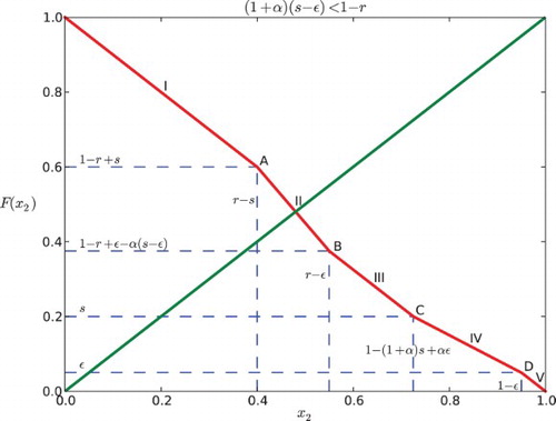
Fig. 3. Return map F for Case I when α=−0.5, s=0.2, r=0.6, and ε=0.05.

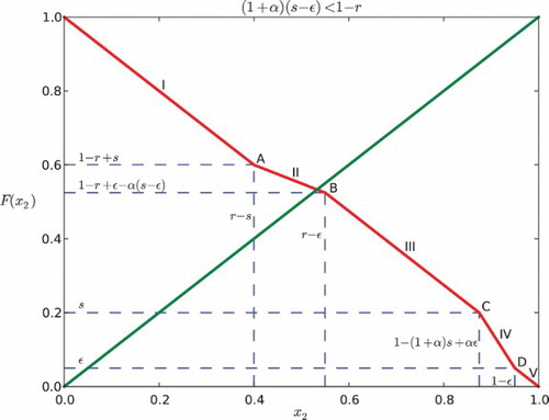
Fig. 4. Return map F for Case II when α=0.5, s=0.4, r=0.6, and ε=0.05.

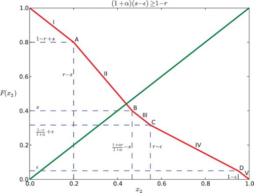
Fig. 5. Return map F for Case II when α=−0.3, s=0.4, r=0.8, and ε=0.05.

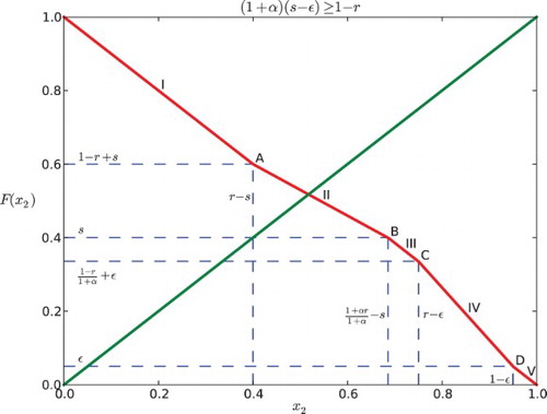
Fig. 6. Regions of parameter space for the k cyclic solutions with k=M+1. Here the feedback is negative with β=−.2 and the gap is ε=0.03. The widest diagonal band contains the parameters for k=2 and is partitioned into six cases. Note that case VI disobeys the constraint ε<r−s. The rest of the diagonal bands contain parameters for k=3, 4, … and each of them is partitioned into five cases.

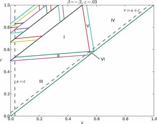
Fig. 7. The number of clusters realized in a cell cycle simulation (a) with no gap and (b) with a gap of ε=0.05 when s≥0.01 and ε=0.5 s when s<0.1. In both plots, the feedback is linear and negative with f(I)=−I. Note the strong agreement between the two plots.

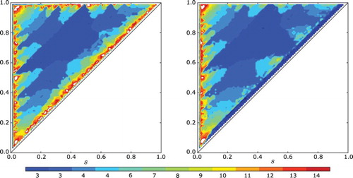
Fig. 8. Clustering of n=120 equi-distributed cells.(a) For s=0.2, r=0.6 and ε=0.03, the cells converge to two clusters. (b) For s=0.2, r=0.8 and ε=0.01, the cells converge to three clusters. For all simulations the feedback was taken to be f(I)=−I. Note in (a) that they first appear to form four clusters, but merge into two clusters.

Fig. 9. Comparison of convergence speed for the model with and without a gap of ε=0.01 and n=60 cells. Norm squared of the gap vector G vs. time. (a) For s=0.2 and r=0.9 both models converge to four clusters. (b) For s=0.3 and r=0.7 both models converge to two clusters. For all simulations the feedback was taken to be f(I)=−I, and the initial condition was evenly distributed – the global minimum for 0. The model with gaps converges to the clustered solutions much more quickly.

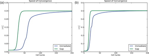
Fig. 10. The final configuration of cells in systems with gap sizes varying in [0.1, 4.9].